MINIMIZATION OF ELECTRICAL LOSSES IN A VECTOR CONTROLLED INDUCTION MACHINE DRIVE

(1)

University of Windsor University of Windsor

Scholarship at UWindsor

Electronic Theses and Dissertations Theses, Dissertations, and Major Papers

2013

MINIMIZATION OF ELECTRICAL LOSSES IN A VECTOR

CONTROLLED INDUCTION MACHINE DRIVE

Debarshi Biswas University of Windsor

Follow this and additional works at: https://scholar.uwindsor.ca/etd

Recommended Citation Recommended Citation

Biswas, Debarshi, "MINIMIZATION OF ELECTRICAL LOSSES IN A VECTOR CONTROLLED INDUCTION MACHINE DRIVE" (2013). Electronic Theses and Dissertations. 4960.

https://scholar.uwindsor.ca/etd/4960

This online database contains the full-text of PhD dissertations and Masters’ theses of University of Windsor students from 1954 forward. These documents are made available for personal study and research purposes only, in accordance with the Canadian Copyright Act and the Creative Commons license—CC BY-NC-ND (Attribution, Non-Commercial, No Derivative Works). Under this license, works must always be attributed to the copyright holder (original author), cannot be used for any commercial purposes, and may not be altered. Any other use would require the permission of the copyright holder. Students may inquire about withdrawing their dissertation and/or thesis from this database. For additional inquiries, please contact the repository administrator via email

(2)

MINIMIZATION OF ELECTRICAL LOSSES

IN A VECTOR CONTROLLED

INDUCTION MACHINE DRIVE

By

D

EBARSHI

B

ISWAS

A Thesis

Submitted to the Faculty of Graduate Studies

through the Department of Electrical and Computer Engineering

in Partial Fulfillment of the Requirements for

the Degree of Master of Applied Science at the

University of Windsor

Windsor, Ontario, Canada

2013

(3)

Minimization of Electrical losses

In a Vector Controlled

Induction Machine Drive

By

Debarshi Biswas

APPROVED BY:

Dr. S. Das, Outside Reader

Department of Civil and Environmental Engineering

Dr. K. Tepe, Departmental Reader

Department of Electrical and Computer Engineering

Dr. N. C. Kar, Advisor

Department of Electrical and Computer Engineering

(4)

iii

AUTHOR'S DECLARATION OF ORIGINALITY

I hereby certify that I am the sole author of this thesis and that no part of this

thesis has been published or submitted for publication.

I certify that, to the best of my knowledge, my thesis does not infringe upon

anyone’s copyright nor violate any proprietary rights and that any ideas, techniques,

quotations, or any other material from the work of other people included in my thesis,

published or otherwise, are fully acknowledged in accordance with the standard

referencing practices. Furthermore, to the extent that I have included copyrighted

material that surpasses the bounds of fair dealing within the meaning of the Canada

Copyright Act, I certify that I have obtained a written permission from the copyright

owner(s) to include such material(s) in my thesis and have included copies of such

copyright clearances to my appendix.

I declare that this is a true copy of my thesis, including any final revisions, as

approved by my thesis committee and the Graduate Studies office, and that this thesis has

(5)

iv

ABSTRACT

Induction motors have found application in household goods as well as in

industries. These machines are rugged and very easy to maintain, making them a favorite

with the consumers. With the introduction of vector control induction motor drives have

gained a lot of popularity. Induction motors, however, prove to be inefficient at low

speeds when compared to other AC machines. Hence there is a need to improve the

efficiency of induction machines over their entire speed range. Thus it is desirable to

design a loss minimization controller which can improve the efficiency. This thesis

therefore documents the following:

 Modeling of an induction motor with core loss included.

 Realization of vector control for an induction motor drive with loss element

included.

 Derivation of the loss minimization condition.

(6)

v

To

My mother and father: Alpana Biswas, Debasish Biswas

My sister: Priyanka Biswas

(7)

vi

ACKNOWLEDGEMENTS

I would like to express my appreciation and sincere gratitude towards my

supervisor, Dr. Narayan Kar for his invaluable support and guidance throughout the

course of this program. His encouragement helped me achieve what was simply an idea

at the beginning of my tenure as a research assistant. He has truly been as inspiration.

Words cannot express the respect I have for him.

I would also like to thank Dr. Kaushik Mukherjee, a visiting professor to

CHARGE labs at the University of Windsor, for his unconditional support during his

tenure here in Windsor. His constant nurturing helped me understand the minute

intricacies that were related to this research. I am indebted to him for sharing his

knowledge with me.

I would like to extend my gratefulness to my committee members, Dr. Kemal

Tepe and Dr. Sreekanta Das, for providing their valuable suggestions and presenting their

insight on my topic of research. Their critiques were indeed helpful in adding value to my

research.

Last but not the least, I would like thank my mother, father, sister and

brother-in-law who stood by me from the moment I started my research. My father has been my

biggest strength as he instilled the confidence in me that I could finish what I started. I

(8)

vii

LIST OF TABLES

(12)

xi

LIST OF FIGURES

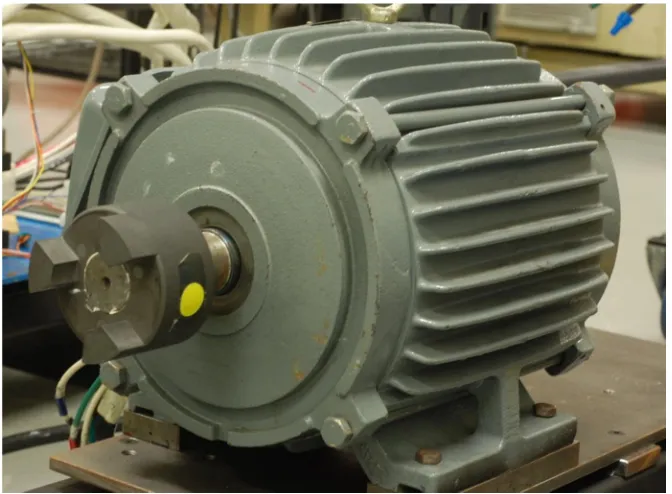
Fig. 1.1. Typical induction motor with cooling fins on the stator and coupler on the

rotor shaft. ...2

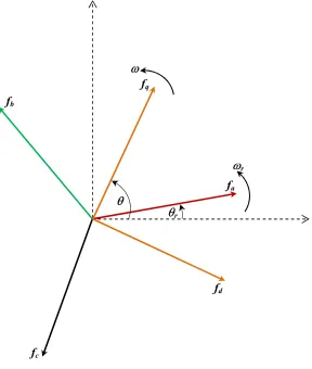
Fig. 2.1. Phasor diagram depicting the positions of three phase values (marked in red, green and black) and the corresponding dq values (marked in orange). . 17

Fig. 2.2. Equivalent circuit of an induction motor. ...18

Fig. 3.1. D. C. shunt motor. ... 21

Fig. 3.2. Orthogonal orientation of armature current and field current in a separately excited DC machine. ...22

Fig. 3.3. Current control loop...27

Fig. 4.1. Dynamic model of an induction motor including core loss...29

Fig. 4.2. Block diagram implementing vector control with core loss included in the modeling. ...31

Fig. 4.3. Representation of a simple feedback loop. ...38

Fig. 4.4. Dynamics of the current control loop... ...40

Fig. 4.5. Outer speed control loop...43

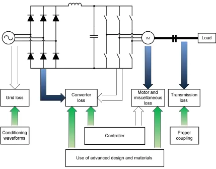
Fig. 5.1. Typical induction motor drive showing the losses incurred by each component (blue arrows) and the methodology used to improve the efficiency (green arrows). ...48

Fig. 5.2. Basic block diagram of a search controller. ...50

(13)

xii

Fig. 5.4. Block diagram of proposed loss minimization controlled induction motor

drive. ...55

Fig. 6.1. Three phase voltage supplied to the induction motor from the grid. ...58

Fig 6.2. Two axis representation of three phase voltage in synchrounously rotating reference frame. ...58

Fig. 6.3. Starting current in an induction motor. ...59

Fig. 6.4. Torque vs. speed characteristics of the 7.5 hp induction motor. ...60

Fig. 6.5. Speed of the induction motor under different loading conditions. ...61

Fig. 6.6. Change in rotor speed due to loading variation from 0% to 50%. ...62

Fig. 6.7. Torque profile of the induction motor under different loading conditions. ...62

Fig. 6.8. Variation in torque when load changes from 0% to 50%. ...63

Fig. 6.9. Variation of stator current under different loading conditions. ...64

Fig. 6.10. Variation of rotor current under different loading conditions ...65

Fig. 6.11. Variation of core loss branch current under different loading conditions. ...66

Fig. 6.12. Variation of magnetizing branch current under different loading conditions.. .67

Fig. 6.13. Change in stator current amplitude due to increase in load from 0% to 50. ...68

Fig. 6.14. Change in rotor current amplitude due to increase in load from 0% to 50...69

Fig. 6.15. Torque profile of the induction motor at full load under vector control. ...70

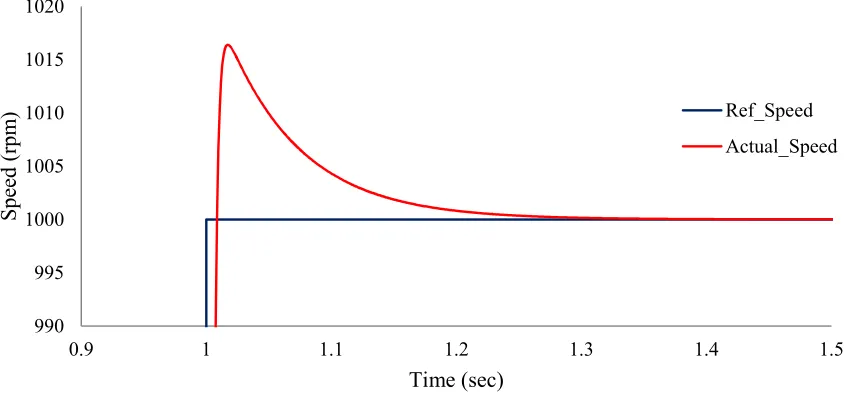
Fig. 6.16. Changes in reference speed as given by the user and dynamics of the actual rotor speed. ...71

(14)

xiii

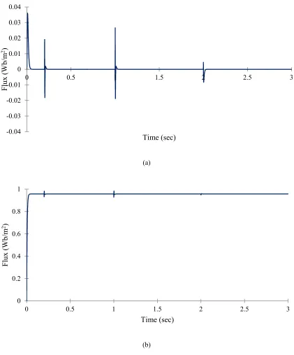
Fig. 6.18. Rotor flux profile as forced by the vector controller. ...72

Fig. 6.19. Time taken to set up rated flux. ...73

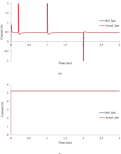
Fig. 6.20. Reference and actual magnetizing currents. ...74

Fig. 6.21. Magnetizing currents in three phase. ...75

Fig. 6.22. Stator currents.. ...76

Fig. 6.23. Stator currents in three phase. ...77

Fig. 6.24. Torque profile under the influence of loss minimization controller. ...79

Fig. 6.25. Reference Speed and dynamics of actual rotor speed. ...80

Fig. 6.26. Reference and actual magnetizing currents. ...81

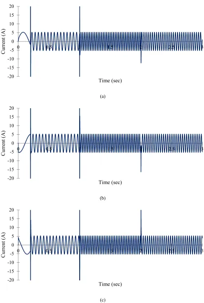
Fig. 6.27. Dynamics of stator current at 1700 rpm.. ...82

Fig. 6.28. Stator currents in three phase at 1700 rpm.. ...82

Fig. 6.29. Dynamics of rotor current at 1700 rpm. ...83

Fig. 6.30. Rotor currents in three phase at 1700 rpm. ...83

Fig. 6.31. Dynamics of core loss branch current at 1700 rpm.. ...84

Fig. 6.32. Core loss branch currents in three phase at 1700 rpm. ...84

Fig. 6.33. Losses in the motor at 1700 rpm. ...85

Fig. 6.34. Reference and actual magnetizing currents at 500 rpm. ...86

Fig. 6.35. Dynamics of stator current at 500 rpm. ...87

(15)

xiv

Fig. 6.38. Rotor currents in three phase at 500 rpm.. ...88

Fig. 6.39. Dynamics of core loss branch current at 500 rpm. ...89

Fig. 6.42. Torque profile under the influence of loss minimization controller ...92

Fig. 6.43. Reference Speed and dynamics of actual rotor speed ...93

Fig. 6.44. Reference and actual magnetizing currents at 1700 rpm.. ...94

Fig. 6.46. Stator currents in three phase at 1700 rpm. ...95

Fig. 6.47. Dynamics of rotor current at 1700 rpm ...96

Fig. 6.48. Rotor currents in three phase at 1700 rpm. ...96

Fig. 6.52. Reference and actual magnetizing currents at 500 rpm ...99

Fig. 6.54. Stator currents in three phase at 500 rpm. ...100

(16)

xv

(17)

xvi

NOMENCLATURE

vqs : Q-axis stator voltage

vds : D-axis stator voltage

vqs_comp : Q-axis compensation voltage

vds_comp : D-axis compensation voltage

iqs : Q-axis stator current

ids : D-axis stator current

iqr : Q-axis rotor current

idr : D-axis rotor current

iqm : Q-axis magnetizing current

idm : D-axis magnetizing current

iqc : Q-axis current in the core loss branch

idc : D-axis current in the core loss branch

qs : Q-axis stator flux

ds : D-axis stator flux

qr : Q-axis rotor flux

dr : D-axis rotor flux

r : Rated flux

(18)

xvii

Rr : Rotor resistance

Rc : Core loss resistance

Lls : Stator leakage inductance

Llr : Rotor leakage inductance

Lm : Magnetizing inductance

Te : Electromagnetic torque

Tl : Load torque

 : Speed of arbitrarily rotating dq-frame rad/sec

r : Rotor speed in rad/sec

sl : Slip speed in rad/sec

 : Angle of transformation from three phase to two phase

J : Moment of inertia

P : Number of poles

p : Differentiation operator

iKp : Inner loop proportional gain

oKp : Outer loop proportional gain

iKi : Inner loop integral gain

i, o : Damping factor for inner and outer loop respectively

ni, no : Natural frequency for inner and outer loop respectively

(19)

xviii

PSCL : Stator copper loss

PCore : Core loss

PRCL : Rotor copper loss

idm_opt : Optimal d-axis magnetizing current

fa, fb, fc : Component of any variable in phase A, B or C respectively

fq, fd : Component of any variable in q or d-axis respectively

(20)

1

1. INTRODUCTION

1.1. I

NTRODUCTION TO

I

NDUCTION

M

OTOR

With the inception of AC distribution systems, application of AC motors has

widened to a large extent. This has prompted motor manufacturers to build AC motors

that will cater to the various types of applications. All electric motors transform electric

power into mechanical power. In DC motors, there is a physical connection between the

stator and the rotor. This allows the transfer of power. However, in AC motors there is no

such physical connection between the stationary and the rotating part. The conversion of

electrical to mechanical energy occurs through induction and hence the name induction

motors. Induction motors are found in many applications today, whether it be in small

scale or large scale. Because induction motors are constant speed motors, they are found

in many household appliances such as pumps and fans. In industries they are used for

heavy duty applications. Induction motors are the largest consumer of electrical power

[1]. The reasons for this popularity are rugged construction, low maintenance cost,

reliable and inexpensive compared to other motors. But possibly the biggest advantage is

that it does not need any starter motor and it can be directly connected to a power source.

It does however have disadvantages. An induction motor works best when it is running at

or near its rated loading capacity. The motor can still be used at lower loading conditions

but at the cost of efficiency. Energy consumption has become an issue over the past few

years. It is of utmost importance that attention is paid to make machines run more

efficiently. Speed control can bring about significant energy savings but vector controlled

induction motor drives focus mainly on delivering high dynamic performance. Thus, it is

(21)

2

compensating for efficiency. Advancements in the design process and improvements in

materials used to construct induction motors have helped improve the efficiency of

induction motors. However, there is no substitute for a controller dedicated to optimize

the efficiency. Loss minimization can be achieved in many different ways. The ideal loss

minimization controller should not only reduce the heat signature of the motor but also

account for losses in the converter in conjunction with delivering the required load

torque. Designing a loss minimization controller will definitely help overcome the

primary disadvantage of induction motors.

Fig. 1.1: Typical induction motor with cooling fins on the stator and coupler on the rotor shaft.

1.2. C

ONSTRUCTION AND

O

PERATION OF AN

I

NDUCTION

M

OTOR

An induction motor is made up of two major components. The outer stationary

casing is called the stator. The stator is made up laminated stamping slotted to hold the

(22)

3

specific number of poles. There are two kinds of rotors for the induction motors. They are

the squirrel cage rotor and the wound rotor. The squirrel cage rotor essentially has metal

bars shorted at the ends by metal rings called the end rings. This construction makes the

rotor look like a squirrel cage and hence the name. Because this kind of a construction

lacks any physical wiring, there is no access to the rotor. This feature makes squirrel cage

motors very rugged and usable in almost any condition. The wound rotor, as the name

suggests, has windings in the rotor which are a mirror image of the windings in the stator.

These motors are used in specific applications due to the access to the windings.

However, wound rotor machines have reliability issues when compared to squirrel cage

machines and are more expensive. In this thesis only the squirrel cage induction motor

will be considered.

An induction motor is essentially a transformer with a rotating secondary.

Exciting the stator windings creates a rotating flux. The speed at which the rotating flux

rotates is called the synchronous speed. The rotating flux cuts across the rotor bars and an

e.m.f. is induced in the stationary rotor as per Faraday's law. The magnitude of this

induced e.m.f. is proportional to the relative velocity between the rotating flux and the

rotor bars. Because the rotor bars are short circuited, a current is produced due to this

induced e.m.f. The direction of this current, as per Lenz's law, is such that it opposes the

cause that produces it. The cause in this case is the relative velocity between rotating flux

and the rotor bars. In order to oppose this cause the rotor begins to rotate in the in same

direction as the rotating flux. It should be noted that the rotor can never catch up to the

rotating flux. If this happened there would be no relative motion between the flux and the

(23)

4

induction motor is always less than the synchronous speed. The difference in of these two

speeds is known as the slip speed which is generally expressed as a percentage of the

synchronous speed [2].

1.3. E

VOLUTION OF

I

NDUCTION

M

OTOR

D

RIVES

Before vector control was developed for induction motors, scalar control was

widely used in speed control of these machines. Perhaps the most popular strategy is the

volts/hertz method. Although scalar control is simple it has a few drawbacks. The biggest

disadvantage of this method is that it has slow transient response time. This means that it

is slow to transition from one operating point to another. In case of any disturbance it is

slow to recover to its original operating point as well. The second flaw of this strategy is

that the slightest of change in supply can upset the air gap flux of the machine which will

in turn affect the speed of the motor. Overall, it can be concluded that scalar control is not

very precise. Some industrial applications may not need such precise speed of operation

but there are many applications that need higher performance drives. F. Blaschke

proposed a revolutionary idea which changed the way induction motors were controlled

[3]. Separately excited DC motors have naturally decoupled armature and field flux. As a

result DC motors have very quick transient response. With the advent of vector control,

AC machines, like the induction motor, could also be made to behave like a separately

excited DC motors. An analogy between the two has been drawn in the subsequent

chapters. Vector control or field oriented control (FOC) was an immense step forward in

terms of performance. Realization of FOC in real-time also became a possibility with the

(24)

5

1.4. L

ITERATURE

R

EVIEW

Strategies to control loss minimization can be broadly classified into two

categories: loss minimization controller and search control. Loss minimization controller

utilizes the machine parameters to estimate the loss model. The controller thus designed

using this procedure is then responsible for selecting an appropriate flux level which

facilitates the minimization of losses. Much research has been conducted in this field

using this strategy [4-13]. Earlier, scalar control was the most widely used technique to

control the speed of induction motors. Scalar control essentially employs choosing a

specific stator voltage and a frequency to facilitate speed control in the induction

machine. For a given operating point for an induction motor there are combinations of

stator voltages and frequencies that exist which promote loss minimization. This has been

very aptly described in [4, 5]. Another method to achieve optimum efficiency has been

presented by H. G. Kim et al. in [6] by using a current source inverter. It was suggested

that the optimum efficiency could be achieved for a specific combination of torque and

speed by reducing the air gap flux. As a current source inverter is being used the air gap

flux can be expressed as functions of stator currents and rotor slip. In addition to reducing

the losses, this method also improved the power factor at light loads. The relationship

between the stator current and the slip frequency, the condition for loss minimization,

was obtained numerically. The control loop was then designed based on these

calculations to accommodate for variable flux. Kioseridis et al. [7] presented a loss

minimization scheme using the loss model of an induction motor. The scheme is simple

and employs optimal air gap flux to achieve loss minimization in scalar controlled

(25)

6

of the drive at a bare minimum. P. Famouri and J. J. Cathey [8] proposed a closed loop

control technique using per unit values. The modeling of the losses was done using the

copper losses, core loss, losses crossing the air gap and the rotational losses. These were

then used to calculate the per unit efficiency as a function of slip and frequency.

Implementation of the closed speed loop was a significant improvement over the previous

open loop volt/hertz technique. Lorenz and Yang [9] proposed a dynamic programming

method which would enhance the efficiency in a field oriented induction motor drive

being operated in a closed cycle. Losses taken into account were the copper and core

losses. The copper loss was expressed as a function of the square of the currents. The

core loss on the other hand was modeled as a function of frequency, exhibiting the

hysteresis and eddy current losses distinctively. The loss of the drive was also considered

and defined as an objective function. The constraints of the objective function were the

limits on motor flux, speed, voltage and current. The optimal trajectory for the flux and

flux producing current were computed by solving the problem. The entire control strategy

was then implemented using a microcontroller. Garcia et al. [10] proposed a novel

method to minimize copper losses and iron losses in variable speed variable torque

induction motor drive while maintaining a good dynamic response. It has been very

clearly stated that a good control over the magnetic flux would result in obtaining a

balance between the copper and iron losses. This balance between the copper loss and

core loss would essentially assist in achieving optimum efficiency. The induction motor

model been expressed in dq-coordinate system. However, for simplicity, the leakage

inductance was deleted from the motor model. Resistances were used to represent the loss

(26)

7

condition for minimum loss where the d-axis current was made the control variable as

this component of stator current would eventually influence the flux level in the induction

motor. Chakraborty and Hori [11] approached the problem of loss minimization from

different perspective altogether. They proposed a hybrid scheme to address this issue

which consisted of combining loss model approach and search control approach in a

vector controlled induction motor. The loss model approach calculated the optimum flux

level numerically. The search control algorithm on the other hand estimated the optimum

flux level based on the measurement of the input the power through an iterative process.

Combining both the loss minimization techniques gave rise to the development of a very

capable controller. The hybridization of the two loss minimization methods ensured that

the controller had a fast response by virtue of the loss model approach. Also, the search

algorithm provided sufficient immunity to variation in motor parameters. Although the

performance of the controller is greatly increased, the approach adopted by the authors in

[11] adds to the complicacy of the overall system. The authors used the same approach to

model the losses as used in [10]. However, a simple and approximate model of the

induction motor to achieve their objective. In [12], the authors, Bernal et al., proposed a

generalized loss model using the dq-theory. This loss model would cater to machines

such as permanent magnet synchronous motors, induction motors, and dc motors which

could be used to the fulfill the needs required in the design procedure of controllers

facilitating to loss minimization. Effects due to core saturation have also been accounted

for by the authors. Interestingly, the loss model proposed in [10] has again been used to

the model the induction motor losses. S. Lim et al. [13] proposed a model which included

(27)

8

connected a dependent voltage source with the core loss resistor as a part of the

equivalent circuit for the induction motor. Based on their modeling, it was reported that

the findings were aligned to the complete induction motor model when compared to the

data presented by previous researchers.

Search controller works on the principle of minimum input power measurement in

order to choose the optimum flux level [14-19]. Moreira et al. [14] introduced a new

method to implement search control algorithm for induction motors. He proposed that the

third harmonic of the air gap flux could be used to determine the currents responsible for

producing the flux and torque in the machine which could be utilized to maximize the

efficiency of the induction motor. He also used this technique to estimate the speed of the

rotor. Necessary adjustments could be made to the flux producing component of the

stator current to ensure production of minimum input power. Sul and Park [15] proposed

an idea where an induction motor could be more efficient if the value of slip was

appropriately chosen. Their idea discarded the need for sensors required to measure

speed. Instead, the stator voltage and the stator current were used to estimate all the

necessary values, slip speed being one of them. All these values were then stored in a

microprocessor which would essentially serve as a look up table. The control system

would then refer to the look up table and choose the optimum slip by trial and error at

first. The control system would then ensure the induction motor is then operated by

tracking the optimal slip. Kirschen et al. [16] maximized the efficiency of the induction

motor drive by making flux the control variable. The flux command was gradually

decreased in very small steps to get to the point where minimum power was required to

(28)

9

a solution. This is because the step size by which the flux command is reduced is very

small. Again, there is no option but to choose small step size for flux reduction because

sudden variations in flux levels in the motor can cause unwanted pulsations in the torque

profile. In spite of choosing a small enough torque pulsations could not be done away

with as evident from the results published. Sousa et al. [17] extended the work already

presented in [16]. A fuzzy logic based controller was used to achieve maximum

efficiency in an indirect vector controlled induction motor. The fuzzy controller ensured

there was an adaptive decrement in the d-axis current, which would eventually reduce the

flux in the machine. This approach was chosen to speed up convergence as search

controllers in general are slow to converge to a solution. In [16] a fixed step size was

chosen for the reduction of the flux command. However, Sousa et al. manipulated the

step size with the help of fuzzy logic controller. Thus, based on the input power

measurement, the controller would initially choose a suitable step size to reduce the

current signal by. But as the d-axis current approached the optimum value the step size

itself would automatically be reduced by virtue of adaptive control. Also, a feed forward

compensation technique was used to reduce the pulsations in the torque profile. Kim et al.

[18] proposed a strategy to control induction motors which would deliver "maximum

power efficiency" augmented with unexceptional dynamic performance. Their strategy

was to adjust the squared rotor flux as per the requirement dictated by the minimum

power algorithm till the input power was at its minimum. Unwanted torque ripple was

mitigated by decoupling the speed of the motor and the rotor flux. This decoupling action

was achieved with the help of a nonlinear controller. The design process of the controller

(29)

10

of the rotor resistance needed to be very accurate because it would eventually affect the

estimation of the rotor flux. Unfortunately, the resistance of the rotor would change with

changes in the temperature inside the induction motor. This could adversely affect the

estimated value of the flux. As a result, the authors devised an online method to measure

the rotor resistance so that any slight change in its value could be quickly tracked and

accounted for by the controller. Undoubtedly, the adoption of this method was a clear

improvement over the previous methods. However, inclusion of these features in the

algorithm added to the complexity of the overall system. Ta and Hori [19] devised a

novel technique to improve the convergence of search controllers. They developed an

algorithm which would provide the optimum value of the current needed for minimum

loss by employing the "golden section technique". Their proposed strategy provided a

fast convergence without the need for measuring speed or torque. In addition to this, the

controller was immune to variation in parameters. There was however issues related to

the selection of the upper and lower limits of the current responsible for setting up the

flux.

1.5. P

ROBLEM

S

TATEMENT

From the previous sections it is clear that loss minimization controller has its own

advantages. Firstly, the controller offers fast response. Secondly, opting for this

methodology to implement loss minimization overcomes the issue of torque ripple

completely which is a common problem with search controllers.

Even though there are advantages, loss minimization controller does have flaws.

The very first flaw is in the designing of the controller itself. Design of the controller

(30)

11

the mathematical model dictates the accuracy of the controller. Any approximations made

in the mathematical model of the motor will affect the performance of the controller.

However, it is not always possible to include all the facets of modeling simply because it

adds to complexity of the overall system. An example of approximations made in motor

modeling can be found in [10]. The authors presented an equivalent circuit of the

induction motor where the leakage inductance was ignored. This approximation was

made in order to avoid making the overall system more complex. The same approach was

chosen by the authors in [11, 12].Thus, the design process of the loss minimization

controller always includes a tradeoff between the complexity and accuracy of the system.

Another factor that affects the loss modeling approach is variation in parameters.

As the motor runs the temperature inside it rises. It is a well-known fact that resistance is

a function of temperature. Thus, any fluctuation in temperature will cause the resistance

of any element to change. Due to this phenomenon, factors affecting parameter variation

should be accounted for in the modeling else no matter how accurate the mathematical

model is, in reality the performance of the controller will be affected. In previous works,

such as [13], the parameters of the induction motor have been considered to be constant.

Even though the system may behave perfectly theoretically, practically variation in

parameters due to temperature change will undoubtedly affect the performance of the

system. Online estimation of parameters is a solution to mitigate this issue but the

complexity of the system increases exponentially. However, as mentioned earlier,

incorporating all the minute intricacies to develop a perfect controller would give rise to a

(31)

12

Search controllers on the other hand do not need prior knowledge of the machine

parameters. The issue with search controllers is that they are slow to converge and

produce ripples in the torque profile of the machine. The search controller works on the

principle of detecting the minimum input power. This process is an iterative process

which eventually is the primary reason for slow convergence. Again, because the flux

level gets adjusted in every iteration, the torque also gets affected as a result. Also, while

implementing search control algorithm, adjustment of the flux should be done in

sufficiently small steps. Sudden and large changes in flux can adversely affect the torque

produced by the machine [16].

1.6. O

BJECTIVE OF THIS

R

ESEARCH

Substantial research has been conducted in the field of loss minimization.

Different avenues have also been explored to achieve this [4-19]. In this thesis, the

strategy of loss minimization controller has been adopted.

Various mathematical models of the induction motor have been proposed by

various researchers. Out of these different models the two axis model proposed by P. C.

Krausse is widely accepted. The model he proposed can be very easily derived from the

three phase steady state circuit of an induction motor. There are two primary reasons for

choosing a two axis model. Firstly, with the help of two axis equivalent circuit there are

only two components of the motor variables that need to be taken into consideration, viz.

q-axis and d-axis components. Secondly, for analytical purposes, a suitable frame of

reference can be chosen based upon the type application the induction motor is being

(32)

13

induction motor is operating in the synchronously rotating frame. This reference frame

would be ideal because all sinusoidal variables will appear as DC values. Also, unlike in

[10], his model includes the leakage inductance. The biggest flaw of using such an

equivalent circuit is that it lacks the core loss resistor. In order to formulate the loss

model it is most desirable that core loss is also included as a part of the equivalent circuit.

Importance is given to the inclusion of core loss because the primary losses experienced

by the induction motor are copper loss (stator and rotor) and core loss. The other losses

such friction and windage loss are comparatively much lesser than copper and core loss

as a result of which they are neglected.

Once the equivalent circuit of the induction motor has been well established focus

will be shifted to modeling the losses. The copper losses will be modeled as functions of

the square of the current. The core loss on the other hand can be modeled in two ways.

The first method would be to express the iron loss as a function of square of the current.

The other method is to express it as a summation of hysteresis loss and eddy current loss.

In this thesis all the losses will be modeled as functions of square of the current. The total

loss expression will be finally expressed as a function of the magnetizing current. It will

be shown in the later chapters that choosing the magnetizing current as the control

variable will be most convenient in order to implement the control strategy. The next step

would be to derive the condition for minimum loss which is the primary objective of this

thesis.

The second objective of this thesis is to design a proportional and integral (PI)

controller for the system. The PI controller is one of the very basic controllers in

(33)

14

properly a PI controller is capable of delivering commendable performance when

compared to the new age controllers. There are two principle methods by which the gains

of a PI controller can be determined. The first method involves solving a set of equations

to determine the controller gains and the second method is to determine those values by

trial and error. Much research has been done where the gains of a PI controller has been

determined by trial and error method. The issue with this method is that it could be time

consuming to come across a value of the gain that serves the purpose. Again, even if the

gains are determined, it cannot be pointed out for sure that the values chosen are the most

apt for the given system. In this thesis the proportional gain and the integral gain have

been calculated mathematically. Another advantage of the mathematical calculation is

that the method introduces two new variables which dictate the values of the proportional

and integral gain. These two variables are more significant when compared to

proportional and integral gain because it is these performance parameters that dictate how

the system will behave when subjected to a specific input.

1.7. O

RGANIZATION OF THE

T

HESIS

The following chapters of this thesis are organized as follows. Chapter 2

introduces the dq-model of the induction machine. The beginning of the chapter gives a

brief history as to how the transition from three phase to two axis theory came about. It

also helps in learning the method necessary to transform from three phase to two phase.

The chapter ends by introducing all mathematical equations that describes the induction

motor in dq-reference frame. Chapter 3 dives into the details of vector using the machine

equations described in chapter 2. An analogy is drawn between the working principle of a

(34)

15

gives a clearer picture as to why the theory for vector control was developed. The

conditions that govern vector control are stated. The equations necessary to implement

indirect field oriented (IFOC) vector control are then derived followed by the

requirements of the PI controller. Chapter 4 speaks more about the induction motor

model. However, it provides vivid details of the changes needed to incorporate core loss

into the already established dq-model of the induction machine. The equations required to

implement IFOC are derived again to account for the changes brought about by the

inclusion of core loss. The focus then shifts to the design methodology adopted in this

thesis to calculate the gains for the PI controller. Chapter 5 gives extensive details on how

the losses are modeled. With the assistance of this loss model the condition for

minimizing the losses in an induction motor is then derived. The results obtained from

simulations are documented in chapter 6. Finally, chapter 7 presents the conclusion and

(35)

16

2. INDUCTION MOTOR MODELING

2.1. T

WO

A

XIS

T

HEORY OF

M

OTOR

M

ODEL

R. H. Park introduced a method in the late 1920s which enabled the elimination of

time varying inductance from stator equations. This method was however applied to

synchronous machines. Essentially he referred the stator variables to a frame of reference

fixed in the rotor. This method today is popularly known as Park's transformation. In the

1930s however, H. C. Stanley proposed a method which would enable the change of

variables for induction machines. Unlike R. H. Park's transformation, Stanley's method

referred the rotor variables to a fixed stationary frame in the stator. G. Kron suggested

another method whereby time varying mutual inductances of a symmetrical induction

motor were eliminated by referring the motor variables to a reference frame rotating in

synchronism with the rotating magnetic field. This reference frame is called the

synchronously rotating frame. D. S. Berenton employed the change of variables for

symmetrical induction machines from a reference frame fixed in the rotor. In essence this

was the transformation done using Park's transformation but applied to induction motors.

These techniques were developed in order to cater to a particular application.

However, in the1950s it became clear that any real transformation that is used to analyze

induction machines could be generalized. This general solution would help in eliminating

the time varying inductances by referring them to a rotating reference rotating at any

arbitrary angular velocity. It should be noted that when using stator reference frame for

(36)

17 fa fc fb fq fd r   r

Fig 2.1: Phasor diagram depicting the positions of three phase values (marked in red, green and black) and the corresponding dq values (marked in orange).

The following equation shows how the three-phase variables can be expressed in an

arbitrary reference frame.

                                                                             c b a d q f f f f f f 2 1 2 1 2 1 3 2 sin 3 2 sin sin 3 2 cos 3 2 cos cos 3 2 0 (2.1)

It can also be shown that the three phase variables can again be obtained from the

(37)

18

Rs Rr

Lm Llr Lls Vqs iqs iqr iqm

ds ( - r)dr

(a)

Rs Rr

Lm Llr Lls Vds ids idr idm

qs ( - r)qr

(b)

Fig 2.2: Equivalent circuit of an induction motor. A) q-axis. B) d-axis.

                                                                   0 1 3 2 sin 3 2 cos 1 3 2 sin 3 2 cos 1 sin cos f f f f f f d q c b a           (2.2)

In equations (2.1) and (2.2) the variable f could be interpreted as voltage, current or flux

(38)

19

The angular velocity  and the angular displacement  are related as per the

following expression



 dt

 (2.3)

2.2. M

ODELING OF AN

I

NDUCTION

M

OTOR

Any induction motor is governed by the following equations [20].

Voltage equations:

ds qs

qs s

qs Ri p

v     (2.4)

qs ds

ds s

ds Ri p

v     (2.5)



r



dr qr

qr r

qr Ri p

v 0      (2.6)



r



qr dr

dr r

dr Ri p

v 0      (2.7)





qr dr dr qr



m

lr m

e i i

L L

L P

T  

 

4 3

(2.12)

r l

e p

P J T

T   2 

(40)

21

3. VECTOR CONTROL OF INDUCTION MOTOR

3.1. T

HEORY OF

V

ECTOR

C

ONTROL

Speed control in induction motors, using scalar control techniques, have been

observed since the earliest of days. The preferred control method was volts per hertz

method, alternately known as scalar control of induction motors. However, scalar control

did not have fast response, as sometimes demanded by the user. DC machines, on the

other hand, could provide very fast transient response. Thus, vector control was

formulated in order to make the AC machine behave like a DC machine. The analogy

between the speed control of DC machine and vector control is explained in the next

section.

Fig. 3.1: DC shunt motor.

3.3.1. ANALOGY BETWEEN VECTOR CONTROLLED INDUCTION MOTOR AND SPEED

CONTROL OF A SHUNT DC MOTOR

Before diving into the theory of vector control of an induction motor, the working

principle of a separately excited DC motor should be understood. This is necessary

(41)

22

Ia

If

Fig 3.2: Orthogonal orientation of armature current and field current in a separately excited DC machine.

are two separate currents at work inside a DC motor. One is called the armature current

and the other is known as the field current. The construction of a DC motor, as depicted

in figure 3.1, is such that both the currents are orthogonal to each other. Because the

currents are responsible for producing the armature and field fluxes, it can inferred that

these fluxes will also be orthogonal. This means that if we depict both the armature and

field currents along with the fluxes through a phasor diagram they would be

perpendicular to each other as shown in figure 3.2. From the phasor diagram it can be

concluded that changing any one of the current values will not affect the other. In other

words, it can be said that changes in armature current will not affect the field current or

the field. Again, the armature current, which directly affects the developed torque of a

DC motor, remains unaffected if any change is observed in the field current. This is the

very reason as to why a DC motor has very fast torque response.

The same idea is extended to induction motors. Through vector control, the d and

q-axis currents are decoupled and made orthogonal. In order to make the sinusoidal

variables such as voltages, currents and fluxes appear as DC quantities the induction

motor is considered to be in a synchronously rotating frame. For an induction motor the

q-axis current is analogous to the armature current and the d-axis current is analogous to

(42)

23

current while the d-axis current remains unaffected. Again, the rotor flux, which is a

function of the d-axis current, can be easily controlled by varying the d-axis current itself

while the torque and q-axis current remain unchanged.

3.3.2. FIELD ORIENTED CONTROL

Vector control, alternately known as field oriented control, is one of the modern

control techniques used to control AC machines. This thesis only looks at the

methodology that can be applied to induction motors only. The name, vector control, has

emerged from the fact that the control is achieved in field coordinates. The parameters

that are controlled with the help of this technique are as follows:

 Stator flux

 Air-gap flux

 Rotor flux

Essentially, the voltages, currents and flux linkages are represented in the form of

vectors. With the help of the controller the specific orientation is achieved. Normally,

while trying to implement vector control rotor flux orientation is best choice as it

provides natural decoupling when compared to stator flux orientation or air-gap flux

orientation.

3.3.3. INDIRECT FIELD ORIENTED VECTOR CONTROL

Indirect field oriented control (IFOC) eliminates the use of sensors which are used

to measure terminal voltages and currents to determine the unit vector components cos

(43)

24

[21]. This method is cost effective but any changes in the parameters of the motor while

in operation makes the controller vulnerable to degradation in performance [22].

At the very outset the conditions that govern vector control must be to understood.

There are three main criteria that need to be satisfied:

 dr r, a constant at steady state (3.1)

  0,  0

dt d _qr

qr (3.2)

  0

dt d dr

, when in steady state (3.3)

With the above conditions in mind the equations for vector control can now be derived.

Substituting dr=r, equation (2.8) can be written as



ds dr



m dr lr

r L i L i i

 (3.4)

Simplifying equation (3.4) further yields

r ds m

r r dr

L i L L

i    (3.5)

Where Lr=Llr+Lm

Substituting qr =0 in equation (2.7) and simplifying the same yields

r qs m qr

L i L

i   (3.6)

(44)

25







   0

         dr qr r r ds m r r r p L i L L R (3.7)

Introducing the conditions (3.2) and (3.3) in equation (3.7) reduces it to

ds m r L i

 (3.8)

Again, substituting (3.6) in (2.3) yields

0              qr r sl r qs m r p L i L

R (3.9)

Where_r _sl and introducing the conditions (3.1) and (3.2) in (3.9) gives

lr r qs m r sl L i L R    (3.10)

Substituting (3.1), (3.2),(3.5) and (3.6) in the torque equation numbered (2.9) yields

qs ds r m

e i i

L L P T 2 4 3  (3.11)

The above equations clearly portray the fact that the conditions assumed for

vector control, equations (3.1) through (3.3), indeed decouple the q and d-axis currents. It

can easily be concluded that ids is the flux producing component while iqs is solely

responsible for changes in the electromagnetic torque.

3.4. R

EQUIREMENTS OF THE

PI

C

ONTROLLER

It is clear from the equations presented in section 3.3.3 that the control variables

(45)

26

Changing the values of these currents will enable the user to very quickly change the

torque at a particular set speed. From figure 3.3 it is clear that the voltage equations need

to be expressed as a function of the stator currents. In order to achieve this it is first

necessary to express the stator fluxes in terms of stator currents only. The procedure is as

follows.

First equation (2.5) is considered. It is a function of iqs and iqr. As mentioned

earlier, the control variables are the q and d-axis stator currents. Thus, iqr needs to be

eliminated from the flux equation.

Substituting equation (3.6) in (2.5) eliminates iqr. The flux equation can be rewritten as

qs s qs Li

 (3.12)

Where

m lr r

m ls s

r s

m

L L L

L L

L

 

  

2

1

Similarly, equation (2.6) is a function of ids and idr. Thus, substituting equation (3.5) in

(2.6) yields

r r m ds s ds

L L i

L  

 

 (3.13)

The stator voltages can now be expressed in terms of stator currents. Thus, substituting

(46)

27

+

- RssLs

1 * qm i qm i + - + + comp qs v _{_} qm i PI (a) +

- RssLs

1 * dm i dm i comp ds v _ dm i PI (b)

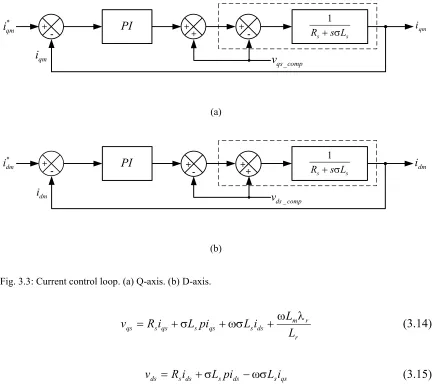
Fig. 3.3: Current control loop. (a) Q-axis. (b) D-axis.

r r m ds s qs s qs s qs L L i L pi L i R

v      (3.14)

qs s ds s ds s

ds Ri L pi Li

v    (3.15)

A close look at equations (3.14) and (3.15) reveals that both the q-axis and d-axis

voltages have dependency on iqs and ids. In other words, the voltage equations are not

decoupled. Considering in vector control, the control variable of choice are the q and

d-axis stator currents, any change in one variable will automatically affect the other. Thus,

the cross coupled terms need to be compensated for. Figure 3.3 shows the procedure by

which the effect of the cross coupled terms can be negated. In equation (3.14) any term

which is a function of ids is treated as a disturbance. Since the magnitude of this

disturbance can be estimated, introducing a signal opposite in polarity but bearing the

(47)

28

equation (3.15), any term which is function of iqs is treated as a disturbance and its effect

(48)

29

4. VECTOR CONTROL OF INDUCTION MOTOR MODEL

WITH CORE LOSS INCLUDED

Rs Rr

Rc

Lm

Llr

Lls

Vqs

iqs iqr

iqc

iqm ds

Lmidm

( - r)dr

(a)

Rs Rr

Rc

Lm

Llr

Lls

Vds

ids idr

idm

idc

qs ( - r)qr

Lmiqm

(b)

Fig: 4.1: Dynamic model of an induction motor including core loss. (a) q-axis. (b) d-axis.

4.1. M

OTOR

M

ODEL

I

NCLUDING

C

ORE

L

OSS

The three phase steady state induction motor model including core loss is well

established [2] and so is the dynamic motor model [20] neglecting core loss. However,

not much attention has been paid to the dynamic model as far as the inclusion of core is

concerned. Considering this thesis deals with minimization of the losses it is of utmost

(49)

30

the model presented in [20] was proposed by [23]. The equations depicting the induction

motor including core loss are depicted by the following equations:

Voltage equations:

ds qs

qs s

qs Ri p

v     (4.1)

qs ds

ds s

ds Ri p

v     (4.2)



r



dr qr

qr r

qr Ri p

v 0      (4.3)



r



qr dr

dr r

dr Ri p

v 0      (4.4)

It should be noted that the voltage has been equated to zero in equation (4.3) and (4.4)

because in a squirrel cage induction motor the rotor bars are shorted with end rings.

Current equations: dm m qm m qc

ci L pi L i

R   (4.5)

qm m dm m dc

ci L pi L i

R   (4.6)

qc qm qr

qs i i i

i    (4.7)

dc dm dr

ds i i i

i    (4.8)

Flux equations:

qm m qs ls

qs L i L i

 _(4.9)

dm m ds ls

ds L i L i

 (4.10)

qm m qr lr

qr  L i L i

 (4.11)

dm m dr lr

dr  L i L i

(50)

31 + - dt d * e

T iqm*

* ds V * qs V qs V ds

V

* r N * dm i qm i dm i qm pi dm pi * r  *  r

N sync*

am

i i_bmicm

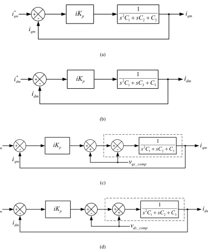
Fig. 4.2: Block diagram implementing vector control with core loss included in the modeling.

Mechanical equations







dr



qs qc



qr



ds dc





m

lr m

e i i i i

L L

L P

T    

  4 3 (4.13) r l e p P J T

T   2  (4.14)

It should be noted here that addition of core loss in the model of an induction motor

increases the order of the system by two.

4.2. I

NDIRECT

F

IELD

O

RIENTED

V

ECTOR

C

ONTROL

In chapter 3 all the necessary expressions for vector control were derived. The

theory essentially remains the same apart from the changes observed in the equations

which will be elaborated in this section. Including the core loss element increases the

(51)

32

longer be chosen as the stator currents. Magnetizing currents are chosen as the control

variables to implement vector control when core loss is included in the modeling of an

induction motor. The block diagram for explaining this method is shown in figure 4.2.

The three main criteria for vector control are reiterated again. They are as follows:

 dr r, a constant at steady state (4.15)

  0,  0

dt d _qr

qr (4.16)

  0

dt d dr

, when in steady state (4.17)

With the above conditions in mind the equations for vector control can now be derived.

Thus, after substituting_dr _r, equation (4.12) can be written as

dm m dr lr

r  L i L i

 (4.18)

From (4.18),

lr dm m r dr

L i L

i   (4.19)

Substituting (4.19) in (4.4) yields







   0

     

   

dr qr

r lr

dm m r

r p

L i L

R (4.20)

Introducing the conditions (4.15) and (4.17) in (4.20) reduces it to

dm m r L i

(52)

33

Substituting (4.16) in (4.11) yields

lr qm m qr L i L

i   (4.22)

Again, substituting (4.22) in (4.3) yields







   0

          qr dr r lr qm m r p L i L R (4.23)

Writing _r _sl and introducing the conditions (4.15) and (4.16) in (2.23) gives

lr r qm m r sl L i L R    (4.24)

Substituting (4.15), (4.16) and (4.22) in the torque equation numbered (4.13) yields





_               lr m qm r m lr m e L L i L L L P T 1 4 3 (4.25)

From the above equations it is evident that the d and q-axis currents have been decoupled

and are completely independent of each other.

4.3. D

ESIGNING THE

C

ONTROLLER

Now that the equations for vector control have been derived, focus should now be

shifted to the requirements of the PI controller. There will be three controllers in used in

the entire system. One PI controller will be for the outer loop or the speed control loop.

MINIMIZATION OF ELECTRICAL LOSSES IN A VECTOR CONTROLLED INDUCTION MACHINE DRIVE

Scholarship at UWindsor

Scholarship at UWindsor

MINIMIZATION OF ELECTRICAL LOSSES IN A VECTOR

MINIMIZATION OF ELECTRICAL LOSSES IN A VECTOR

CONTROLLED INDUCTION MACHINE DRIVE

CONTROLLED INDUCTION MACHINE DRIVE

MINIMIZATION OF ELECTRICAL LOSSES

IN A VECTOR CONTROLLED

INDUCTION MACHINE DRIVE

By

D

B

Minimization of Electrical losses

In a Vector Controlled

Induction Machine Drive

AUTHOR'S DECLARATION OF ORIGINALITY

ABSTRACT

To

My mother and father: Alpana Biswas, Debasish Biswas

My sister: Priyanka Biswas

ACKNOWLEDGEMENTS

TABLE OF CONTENTS

LIST OF TABLES

LIST OF FIGURES

NOMENCLATURE

1. INTRODUCTION

1.1. I

I

M

1.2. C

O

I

M

1.3. E

I

M

D

1.4. L

R

1.5. P

S

1.6. O

R

1.7. O

T

2. INDUCTION MOTOR MODELING

2.1. T

A

T

M

M



2.2. M

I

M

































3. VECTOR CONTROL OF INDUCTION MOTOR

3.1. T

V

C







