ABSTRACT
CHUNG, SEUNG EUN. Designing Practical Mobile Interaction Interfaces through Mobile Sensing. (Under the direction of Injong Rhee and Mladen Vouk.)
Aided by the prevalence of radio-connected, sensor-rich devices such as smartphones, tablets, and wearable devices in everyday life, the realization of ubiquitous computing has become closer than ever. In ubiquitous computing, mobile devices are closely connected to each other and frequently interact with nearby devices. However, contemporary interaction interfaces are inadequate to meet the demands for frequent connectivity. Mobile devices need to interact in an unobtrusive and sensory manner. As a basic enabling technology that builds up the foundations of the new computing paradigm, this dissertation presents new interaction interfaces for mobile systems via an application-driven approach.
First, we envision a virtual trackpad interface that tracks user input on any surface near the mobile device. We adopt the acoustic signal as the medium for interaction, which can be handled by lightweight signal processing using inexpensive sensors on mobile devices. In our prototype named vTrack, the peripheral device simply emits inaudible acoustic signals through a loudspeaker, while the receiving device performs sound source localization by leveraging a multi-channel microphone array. We build a fingerprint-based localization model using various cues, such as time difference of arrival, angle of arrival, and power spectrum density of the audio signal. The vTrack system integrates the frequency difference of arrival incurred by the Doppler shift to track the sound source in motion. Finally, the position estimations are fed into the extended Kalman filter to reduce errors and smooth the output.
© Copyright 2016 by Seung Eun Chung
Designing Practical Mobile Interaction Interfaces through Mobile Sensing
by
Seung Eun Chung
A dissertation submitted to the Graduate Faculty of North Carolina State University
in partial fulfillment of the requirements for the Degree of
Doctor of Philosophy
Computer Science
Raleigh, North Carolina 2016
APPROVED BY:
Khaled Harfoush Mihail Sichitiu
Injong Rhee
Co-chair of Advisory Committee
Mladen Vouk
DEDICATION
BIOGRAPHY
ACKNOWLEDGEMENTS
First, I would like to express my gratitude to my advisor Dr. Injong Rhee for his thoughtful guidance and endless support in all aspects of the research process. Most of all, I value his insight for high-quality research and his patience and understanding over the past several years. I am also deeply grateful to my co-advisor Dr. Mladen Vouk and advisory committees Dr. Khaled Harfoush and Dr. Mihail Sichitiu for serving on my dissertation committee. I appreciate their generosity of time and insightful feedback.
As a member of the Network Research Lab, I would like to thank my fellow labmates for helpful discussions and comments. I thank all of the faculty and staff members in the Computer Science department for their active support towards my research. I feel fortunate to have had opportunities to work at Samsung Research America in San Jose and Samsung Electronics DMC R&D center in Suwon, Korea as an intern. I thank mentors and many other researchers at both locations. I am grateful to my graduate advisor Dr. Chong-kwon Kim at Seoul National University who inspired and prepared me to pursue this degree.
I count myself lucky to have many amazing friends here in Raleigh and also in Korea. I appreciate their constant encouragement and support over these years. Thank you all for always being there and sharing memories throughout my Ph.D. life. Finally, I cannot thank enough my family for their unconditional love and earnest support in every endeavor. Without their inspiration and encouragement amidst difficult times, my doctoral journey would not be possible. This dissertation is dedicated to them.
TABLE OF CONTENTS
LIST OF TABLES . . . vii
LIST OF FIGURES. . . viii
Chapter 1 Introduction . . . 1
1.1 2D and 3D Gesture Tracking for Mobile Devices . . . 3
1.2 Unobtrusive Interaction Interface for Multiple Co-located Devices . . . 3
Chapter 2 A Virtual Trackpad Interface using Sound Source Localization. . . 5
2.1 Introduction . . . 5
2.2 Related Work . . . 8
2.2.1 Sound Source Localization . . . 8
2.2.2 Mobile Input Techniques . . . 10
2.3 2D Sound Source Tracking . . . 11
2.3.1 Coordinate Positioning . . . 11
2.3.2 Movement Detection . . . 18
2.4 Implementation . . . 22
2.4.1 Audio Signal Design . . . 22
2.4.2 Signal Processing . . . 23
2.4.3 Noise Reduction . . . 26
2.5 Performance Evaluation . . . 27
2.5.1 Experiment Setup . . . 27
2.5.2 Static Sound Source Localization . . . 28
2.5.3 Moving Sound Source Localization . . . 30
2.6 Conclusion . . . 33
Chapter 3 3D Motion Tracking through Sound Source Localization . . . 34
3.1 Introduction . . . 34
3.2 Related Work . . . 36
3.2.1 Vision-based Tracking . . . 36
3.2.2 Audio-based Tracking . . . 37
3.2.3 Sensor-based Tracking . . . 38
3.2.4 RF-based Tracking . . . 38
3.3 3D Motion Tracking . . . 38
3.3.1 3D Space Modeling using TDoA . . . 38
3.3.2 Candidate Matching from DB . . . 43
3.3.3 Handling the Moving Sound Source . . . 45
3.3.4 Improving the Accuracy . . . 46
3.4.1 3D Rendering . . . 48
3.5 Performance Evaluation . . . 50
3.5.1 Micro-benchmarks . . . 51
3.5.2 Macro-benchmarks . . . 56
3.5.3 Energy Consumption . . . 58
3.6 Conclusion . . . 59
Chapter 4 An Unobtrusive Interaction Interface for Multiple Co-located Devices . . . 60
4.1 Introduction . . . 60
4.2 Related Work . . . 62
4.3 Coexistence Detection . . . 63
4.3.1 Similarity Feature Extraction . . . 64
4.3.2 Similarity Metric Verification . . . 65
4.3.3 Impact of Signal Fluctuation . . . 69
4.3.4 Impact of the Number of APs . . . 71
4.3.5 Co-located Device Discovery . . . 72
4.4 System Implementation . . . 74
4.4.1 In-phone Processing . . . 75
4.4.2 In-cloud Processing . . . 76
4.5 Evaluation . . . 77
4.5.1 Discovery Performance . . . 77
4.6 Conclusion . . . 79
Chapter 5 Conclusion . . . 80
LIST OF TABLES
Table 3.1 Anthropometric dimensional data of shoulder-to-wrist length in cm. . . 40 Table 3.2 Tracking results according to different tracking time show 3DTrack’s
position estimation error does not accumulate over time. . . 56 Table 3.3 Energy consumption measured during one-hour application run. Case
1 keeps only the screen on. Case 2 turns both screen and audio record-ing function on. Finally, case 3 activates all functionalities includrecord-ing coordinate computation, audio signal processing and filtering. . . 58 Table 4.1 Correlation coefficients between the ground truth and multiple dataset
using different distance metrics. . . 67 Table 4.2 Time to get a Wi-Fi scan result and the corresponding peer discovery
LIST OF FIGURES
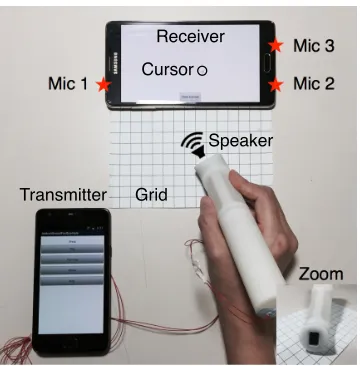
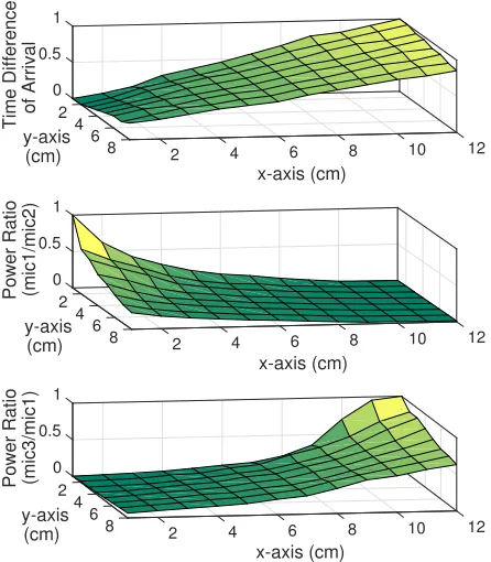
Figure 2.1 vTrack operation scenario using two mobile devices. Receiver records the audio signal using three on-device microphones and visualizes the sound source position by a cursor on its screen. Transmitter emits inaudible (19kHz) acoustic signals repeatedly through an external speaker. User moves the sound source on a virtual trackpad grid. . . 7 Figure 2.2 Normalized time difference of arrival (top) and power ratio values
(middle and bottom) of audio signals recorded by two microphones. Measurements are taken at each point of the grid. . . 12 Figure 2.3 Distribution of cross-correlation index value and power ratio of audio
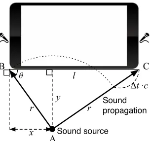
signals measured on two different days (solid lines: first day, dotted lines: second day). . . 13 Figure 2.4 Angle of arrival (θ), range (r), and perpendicular distance (y)
estima-tion using the time difference of arrival (∆t) measure at two micro-phones. . . 15 Figure 2.5 Coordinate estimation of the sound source S(XS, YS) using the
dis-tance to three microphones M1, M2, and M3 presented on a Cartesian coordinate system. . . 16 Figure 2.6 Change in frequency (top) and amplitude (middle) of the audio signal
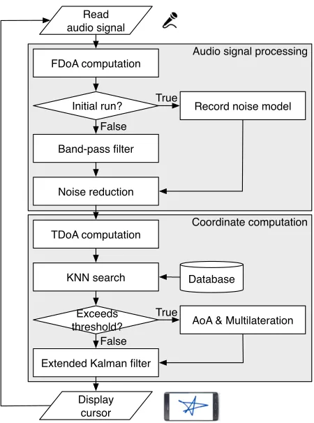
observed by two microphones during the sound source movement. Velocity estimation (bottom) of the moving sound source using the Doppler shift. . . 18 Figure 2.7 vTrack’s operation flowchart on the receiving mobile device. Audio
signal processing module performs frequency-domain analysis on the audio signal. Coordinate computation module obtains various cues from the signal for coordinate positioning. . . 23 Figure 2.8 Sample waveform of 2ms-long sine signal emitted every 21ms by the
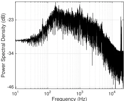
transmitting device. . . 24 Figure 2.9 Ambient noise measured at a local Starbucks cafe. Various machine
sounds result in a high-frequency (∼19kHz) background noise. . . 26 Figure 2.10 vTrack’s noise reduction procedure builds a noise model by
record-ing the background noise and performs spectral subtraction on the original audio signal through frequency-domain analysis. . . 27 Figure 2.11 (a) Angle of arrival and (b) range of the sound measurements with
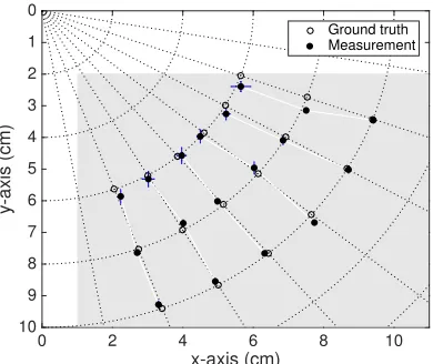
various angle and distance parameter combinations. All error bars stand for standard deviation. . . 28 Figure 2.12 Measurement points and results presented using the angle and range
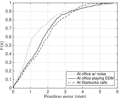
Figure 2.13 Distribution of position estimation error in (a) static and (b) moving sound source scenarios. . . 30 Figure 2.14 Tracking results composed of straight line and curve movements. . . 31 Figure 2.15 Distribution of position estimation error with a moving sound source
in different background noise scenarios. . . 32 Figure 2.16 Two additional input applications using vTrack system: (a) a larger
virtual trackpad workspace with 20×26cm grid size, (b) an Apple key-board layout printed on 18×8cm paper. . . 32 Figure 3.1 3DTrack’s application scenario for a virtual reality (VR) device setting. A
head-mounted mobile device tracks the movement of sound-emitting wearable devices such as smart watches. . . 35 Figure 3.2 Experimental setup of 3DTrack using a 3D cuboid testbed. Receiving
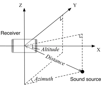
device is attached in front of the cuboid workspace, while the sound source is allowed to move inside of the cuboid. . . 39 Figure 3.3 3D coordinate of a sound source is defined by altitude, azimuth angles,
and distance from the receiving mobile device. . . 40 Figure 3.4 Distance differentials between theoretical distance and actual
mea-surement depending on distance, azimuth, and altitude parameters. All error bars indicate standard errors. . . 41 Figure 3.5 Modeling results of 3D workspace database using theoretical time
difference of arrival values computed by different pair of microphones. 42 Figure 3.6 Time difference of arrival measures by two microphones 1 and 2 can
localize a sound source on a surface (hyperboloid 1) in 3D space. With three microphones, the position is identified on a line (shown in red), which is the intersection of two hyperboloids 1 and 2. . . 43 Figure 3.7 Index estimation result of k-nearest neighbor matching when using
time difference of arrival measures applied to the 3D database in a static sound source scenario. . . 44 Figure 3.8 Candidate selection algorithm of moving sound source scenario. Based
on the inverse distance law of sound, change in sound amplitude is used to infer the distance of sound source from the receiver. . . 45 Figure 3.9 Azimuth and altitude angle of arrival computation in 3D using the
time difference of arrival (∆t) measure at two microphones. . . 47 Figure 3.10 Distribution of azimuth and altitude angle estimation error in 3D. . . . 47 Figure 3.11 3D perspective projection for 3D rendering on a 2D screen. Sound
source P in 3D workspace is projected onto 2D surface S (S’) from the observer’s eye position E in 3D. . . 49 Figure 3.12 Tracking results showing movements with minute differences in
Figure 3.13 Distribution of position estimation error for 3D tracking. 3D measure includes three-axes performance, while 2D measure computes accu-racy for only two axes. . . 51 Figure 3.14 Raw tracking data and calibrated tracking result by applying extended
Kalman filter. . . 52 Figure 3.15 Tracking results performed on a virtual surface in three-dimensional
space and their projection results on a two-dimensional plane. . . 52 Figure 3.16 Distribution of position estimation error with different x, y, and z-axis
parameters. . . 53 Figure 3.17 Distribution of depth estimation error compared to the ground truth
depth change during the movement. . . 54 Figure 3.18 Distribution of distance estimation error compared to the ground
truth distance traveled during the movement. . . 55 Figure 3.19 3DTrack’s tracking results compared with Kinect motion sensor. . . 57 Figure 3.20 Distribution of position estimation difference between 3DTrack and
Kinect motion sensor. . . 57 Figure 4.1 Experiment setup in an engineering building. 116 measurement points
(corridor: labels 1∼56, classroom 1: labels 57∼72, classroom 2: labels 73∼88, classroom 3: labels 89∼116) are spaced 2.4 meters apart. Each color maps a color-labeled AP and its signal coverage, while black-labeled APs are targeted to cover each classroom they are located. . . 65 Figure 4.2 Proposed similarity metric and the Spearman rank-order correlation
computed between point 1 and all other points in the corridor. . . 66 Figure 4.3 Heatmaps of (a) the physical distance and (b) dissimilarity measures
between all measurement points in the corridor. . . 67 Figure 4.4 Heatmap of similarity measure for measurement points in the corridor
(labels 31∼56) and the adjacent classrooms (labels 57∼116). . . 68 Figure 4.5 Distribution of moving standard deviation of RSS for three different
window length. . . 69 Figure 4.6 Distribution of similarity measure between two Wi-Fi scans performed
within various window length. . . 70 Figure 4.7 Distribution of similarity measure between the reference RSS reading
and different number of cumulative scan results. . . 71 Figure 4.8 Impact of the number of overlapping APs and their RSS in dBm to the
similarity index. . . 72 Figure 4.9 Hierarchical clustering result using the proposed threshold strategy in
Figure 4.10 Server collects Wi-Fi signature from clients and clusters them by com-puting similarity of signatures. Then, the server connects clients in the cluster using messaging protocol. Clients perform Wi-Fi scan and communicate over the network. . . 75 Figure 4.11 Number of devices discovered in the same group and success ratio of
Chapter
1
Introduction
Mobile devices are a pervasive part of our everyday life. In ubiquitous computing, mobile devices are closely connected to each other and frequently interact with nearby devices. These pervasive devices affect the way we interact, share, and communicate with other people as well as other devices.
Mobile interaction studies these new aspects of interaction on mobile devices, which have many factors that differentiates them from traditional personal computing by their small sizes, ubiquitous uses, and frequent connectivity. In this dissertation, we focus on two representative aspects of mobile interaction: control mobile devices through their input modalities, and share data and communicate with other devices.
We pinpoint limitations regarding these two factors. First, the small-size input interface of mobile devices limits the user experience in controlling them. For example, software keyboards are error-prone due to their small sizes compared to the size of one’s fingers. Also, fingers themselves block the touchscreen during the interaction. Second, mobile interaction demands a sensory and non-intrusive connectivity, because current methods involve time-consuming steps for searching and selecting the target device in the scan results. Also, dedicated and compatible hardware equipped on both devices are required to establish connection, where delicate physical conditions need to be met. For example, NFC provides 10 centimeters of communication range, while Bluetooth supports 30 centimeters to establish one-to-one connection between two nearby devices.
are some Bluetooth keyboards that allow typing input, while smartpens let users take notes on any surfaces near the device. Regarding the connectivity between devices, many applications in the app store establish connection using various cues, which recognize simultaneous gesture events to share the data. For example, bumping or shaking mobile devices at the same time allows users to exchange their name cards or pictures.
We pay attention to the advancements in mobile device hardware especially the sensors. Modern audio sensors allow high definition sensing on mobile devices. Stereo recording is available by leveraging multi-channel microphones. Active noise cancellation with dedicated microphone is supported to enhance the quality of phone calls. Also, most mobile devices use 24-bit audio data with 192 kHz audio sampling rate, which is 4 times of performance enhancement that is recently made in terms of the audio sampling rate. Additionally, a high-quality loudspeaker produces flawlessly clean audio output. Wireless sensing module provides fast and low-power dualband sensing. We find that many of the challenges in mobile interaction can be overcome by adopting sensing capability of mobile devices.
This dissertation aims to realize mobile interactions through mobile sensing on off-the-shelf mobile device by using the minimum set of on-device sensors. We achieve our goal via light-weight real-time processing, in terms of both computation and power consumption of device. Obviously, the proposed methods accomplish high accuracy in delivering user’s intention for interaction. We propose three practical mobile interaction interfaces. First, we present near-device two dimensional sound tracking by sound source localization technique. Second, we extend it to three dimensional space and achieve 3D motion tracking using acoustic signals. Finally, proximity detection technique for multiple co-located devices is proposed.
new technology.
1.1
2D and 3D Gesture Tracking for Mobile Devices
Although touchscreens on mobile devices allow intuitive interactions through haptic com-munication, the user experience is limited by the size of two-dimensional touchscreens. By adopting audio sensors such as a speaker and multi-channel microphones that are already embedded on mobile devices by default, we extend the range of mobile interaction from touchscreens to any surfaces near the device. Additionally, we stretch the scope from a two-dimension surface to a three-dimensional space.
In Chapter 2, we propose vTrack[9], a virtual trackpad interface that tracks the user’s input movements near the mobile device. We build our system based on the sound source localization technique using the acoustic signal for interaction, because it does not require any expensive sensors or additional resources on mobile devices. We demonstrate that various characteristics of audio signal can be applied in the context of mobile interaction and propose a novel coordinate positioning algorithm that achieves millimeter-level tracking accuracy.
In Chapter 3, we extend the vTrack system to track the sound source in a three dimensional space. Our audio-based 3D tracking approach compensates the limitation of the vision-based motion tracking, which has a limited field of view confined by the camera’s angle. By adopting additional cues including the inverse distance law and Doppler effect of the sound, we reduce the ambiguity in inferring the depth information of the sound source in a three dimensional space and accomplish continuous 3D motion tracking with high-accuracy.
1.2
Unobtrusive Interaction Interface for Multiple Co-located
Devices
Customary device configuration for establishing connection among devices usually ma-nipulate the device identifier uniquely associated with the recipient. These methods involve mundane steps of searching and specifying the receiver, which consume both considerable time and effort to initiate the communication. It definitely degrades the handiness of the service, and will increase nuisances specifically when used by ubiquitous devices that incur frequent networking. This induces the need of a new interaction interface design.
Chapter
2
A Virtual Trackpad Interface using Sound
Source Localization
Touchscreens on mobile devices allow intuitive interactions through haptic communication, but their limited workspace confines user experiences. In this chapter, we envision a virtual trackpad interface named vTrack that tracks user input on any surface near the mobile device. We adopt the acoustic signal for the interaction, which can be handled by lightweight signal processing using inexpensive sensors on mobile devices. In our vTrack prototype, the periph-eral device simply emits inaudible acoustic signals through a loudspeaker, while the receiving device performs sound source localization by leveraging a multi-channel microphone array. We build a fingerprint-based localization model using various cues, such as time difference of arrival, angle of arrival, and power spectrum density of the audio signal. The vTrack system integrates the frequency difference of arrival incurred by the Doppler shift to track the sound source in motion. Finally, the position estimations are fed into the extended Kalman filter to reduce errors and smooth the output. We implement our system on Android devices and validate its feasibility. Our extensive experiments show that vTrack achieves millimeter-level accuracy in the moving sound source scenario.
2.1
Introduction
fingers. The major inconvenience incurred by the touch input is the finger itself, which blocks the screen during the interaction. Therefore, we focus on the aspect that any surface near the mobile device can operate as a virtual trackpad, if user’s movement can be accurately traced. Using this virtual trackpad, users can manipulate the mobile device from outside the touchscreen, without blocking the view of the screen; for example, they can rewind or fast-forward a video while playing it or control characters during the mobile games.
In this chapter, we envision vTrack, a virtual trackpad interface that tracks the user’s input near the mobile device, which extends the range of mobile interaction over the touchscreen. We build the system based on sound source localization technique using the acoustic signal, because it neither requires expensive sensors nor computation-intensive processing on mobile devices. In addition, our system design does not utilize explicit networking between the peripheral and receiving device, because the peripheral does not transmit any data to the receiver; rather, it only emits the sound signal. This excludes any networking module on the peripheral and allows the system to maintain as minimal resource as possible. Low computing and communications on device consequently results in low power consumption, which meets the most significant requisite of peripheral devices.
For the proof-of-concept, we use an off-the-shelf mobile device as the peripheral, which functions as an input device held by a user. Furthermore, we design and build a pen-shaped peripheral using a 3D printer to enhance the usability. In further stages of production, any type of wearable devices with a speaker including smart watches and rings may adopt vTrack to allow ubiquitous interactions with mobile devices. As the peripheral is equipped with a speaker that only costs a few dollars, we expect drastic reduction of the product price when commodified.
The receiving device detects the audio signal and performs sound source localization on-device in real-time. The signal processing and localization procedures are entirely managed by the receiver by taking advantage of its relatively abundant computing resources compared to the peripheral. It uses three-channel built-in microphones that come with a modern smartphone: a primary microphone is for voice recording purposes, while other two are intended to perform stereo recording and cancel the background noise. Figure 2.1 shows vTrack’s operation scenario using two mobile devices. An external speaker peripheral is connected to the transmitter device.
Mic 1 Mic 2 Mic 3
Zoom Receiver
Transmitter Grid
Speaker Cursor
Figure 2.1 vTrack operation scenario using two mobile devices. Receiver records the audio signal us-ing three on-device microphones and visualizes the sound source position by a cursor on its screen. Transmitter emits inaudible (19kHz) acoustic signals repeatedly through an external speaker. User moves the sound source on a virtual trackpad grid.
Our assumption that the peripheral device has an asymmetric capability compared to the receiver device differentiates our work from others in the literature. It limits the system to perform one-way sensing in a synchronization-free manner, with no additional cues for localization other than the sound signal. Second, the audio sampling rate is bounded to 192kHz at driver- or operating system-level on mobile devices, which limits the positioning granularity to 1.8mm when solely relying on the time difference of audio samples. Finally, the moving sound source increases the uncertainty involved in the acoustic sensing, due to various reasons such as multipath reflections and variance in the signal direction.
accuracy.
We have implemented vTrack using two Android devices. Our experiment verifies that combinations of the aforementioned cues are sufficient to resolve the challenges and envision sound source localization with high accuracy. The AoA of the sound measurements are also noticeable: 0.8◦ of angle estimation error and 1.1mm of range estimation error. In
general, vTrack achieves 1.1mm positioning accuracy in moving sound source scenario, which surpasses the theoretical granularity limited by current audio sampling rate. These promising results demonstrate the potential of vTrack in sound source localization-based mobile interactions.
This chapter is organized as follows. Section 2.2 reviews previous work in sound source localization and mobile interaction literatures that are closely related to the prosed system. Section 2.3 describes the underlying core ideas of our system and validates its feasibility. Section 2.4 discusses signal processing and implementation details, and Section 2.5 presents performance of the system based on our extensive experiments. Finally, Section 2.6 concludes the chapter.
2.2
Related Work
In this section, we first summarize related work that performs sound source localization in different scenarios. Then, we introduce various near-device mobile input techniques proposed in the literature, as well as commercial devices in the market.
2.2.1
Sound Source Localization
There exists significant research on acoustic signal-based positioning techniques. We catego-rize these techniques into two groups by the scope of their target scenario.
2.2.1.1 Large-Scale Localization Scenarios
Recently, peer-assisted acoustic ranging scheme[29]is proposed to improve the localization errors induced from the intrinsic limit of the RF signal propagation. Also, PANDAA[52] determines the relative locations of networked sensors measuring the time difference of arrivals of ambient sound in the room. Aforementioned systems aim to localize the object in large-scale indoor scenarios (i.e., building or room-size environments), while our operation space is bounded to tablet-size range.
Other acoustic localization schemes mainly targeted for outdoor environments include ENSBox[12], which is an angle of arrival-based distributed system integrated on ARM plat-form with four-channel microphones at each node. By virtue of its relatively abundant microphone array that is geometrically arranged in 3D space, it achieves high accuracy in object positioning, up to few centimeters. Whistle[59]leverages the time difference of arrival of the acoustic sound observed at different receiving devices, which serve as the basic infras-tructure of the system. Finally,[61]classifies the position of device in a car to detect driver phone use by analyzing the TDoA of acoustic signals emitted from four-channel built-in speakers.
2.2.1.2 Small-Scale Localization Scenarios
Our work is closely related to proposals that study ranging between nearby devices. Beep-Beep[40]is an acoustic ranging mechanism that operates on off-the-shelf mobile devices. Two devices emit a beep sound in turn and simultaneously record both beep sounds. From the (self ) audio recording, each device can measure the elapsed time between two beep sound events. By exchanging this time information, devices can obtain the time of flight of the two beeps, and consequently get the distance between two devices. BeepBeep assumes two mobile devices to have equivalent computing capability, and coordinated with wireless communications such as Wi-Fi or Bluetooth. Its ranging accuracy exceeds one centimeter, which is inappropriate for applications that require precision.
Based on the BeepBeep procedure,[45]extends the phone-to-phone localization to three-dimensional space. By leveraging multiple microphones and other inertial sensors on mobile devices, it performs 3D triangulation using time of arrival and signal power of the acoustic signal. Through continuous localization, each device can estimate the other device’s relative position and track its movement. However, this work aims for a meter-level operation range, and achieves 3D localization accuracy with several centimeters of position error. Similarly,
devices, which enables phone-to-phone motion games.
2.2.2
Mobile Input Techniques
Various types of mobile input methods have been proposed recently, which refrain from direct interactions with the touchscreen due to the inherent limitations of touch interface. UbiK[55] is a portable text-entry method that requires a keyboard outline printed on a paper. It makes use of the dual-microphone interface on a mobile device to localize the keystroke sound on solid surfaces such as desk. UbiK copes with the acoustic multipath fading through Amplitude Spectrum Density (ASD) of different keystroke sound, and localizes distinct keystroke locations by fingerprinting-based signature matching. This scheme is highly dependent upon the surface environments it works on, and demands of repetitive training process every time when the workspace changes. Similarly,[30]snoops keystrokes behind the keyboard based on the TDoA and other acoustic features.
Okuli [63] takes Visible Light Sensing (VLC) technology into account to let the VLC-capable mobile device to sense the movement of user’s finger. It extends the mobile interac-tion workspace to nearby surfaces and enables a virtual trackpad and keyboard input. Using an LED transmitter and two photodetectors as peripherals, Okuli builds a model-driven framework based on the physical properties of the visible-light channel for finger position-ing. It achieves around one-centimeter scale precision, but requires a specially designed peripheral equipped with additional sensors. Other than visible light, the uses of RFID tag and receivers[54]and inertial motion sensors[2, 60]for handwritten text in the air have been proposed for mobile input.
their high price range–from $100 to $200–due to the adoption of various expensive sensors and computing resources to achieve a high level of accuracy when determining the position of the pen.
2.3
2D Sound Source Tracking
vTrack is composed of two mobile devices as illustrated in Figure 2.1. Receiving device is placed horizontally to perform audio signal processing and display the cursor on screen along with the user’s movement. The peripheral periodically emits audio signals, and is allowed to move around on the virtual trackpad printed on a piece of paper, which is a 10×13 grid with 1cm unit. We verify later through experiment that the size of the virtual trackpad is not necessarily limited to the distance between microphones, but can be enlarged to twice its current size.
2.3.1
Coordinate Positioning
2.3.1.1 Time Difference of ArrivalMultilateration is a common navigation technique based on the measurement of the differ-ence in distance to two known locations. Because it utilizes the relative differdiffer-ence instead of the absolute distance measures, it is free from clock synchronization between the signal transmitter and its receiver. We benefit from this property to build a synchronization-free one-way sensing system, and use the Time Difference of Arrival (TDoA) of sound for coor-dinate localization. For TDoA computation, we adopt Generalized Cross Correlation with Phase Transform (GCC-PHAT) algorithm[24], which is known to effectively reduce the noise and reverberation and perform well in actual noisy environments[5]. The index count of the maximum absolute value of GCC-PHAT is considered as the time lag between two audio signals.
Time Difference of Arrival
y-axis (cm)
0 0.5
2 1
4 6
x-axis (cm)
8 2 4 6 8 10 12
y-axis (cm)
Power Ratio (mic1/mic2) 0
0.5
2 1
4 6
x-axis (cm)
12
8 2 4 6 8 10
y-axis (cm)
Power Ratio (mic3/mic1) 0
0.5
2 1
4 6
x-axis (cm)
8 2 4 6 8 10 12
Figure 2.2 Normalized time difference of arrival (top) and power ratio values (middle and bottom) of audio signals recorded by two microphones. Measurements are taken at each point of the grid.
measurement results collected on a different day, and we can observe that cross-correlation index values at the same point are consistent over time and thus reproducible.
Based on this consistency, we first perform linear regression on the measurement data and model the relationship between TDoA and the x-coordinates (i.e., left-right). However, because TDoA is a relative difference measure, locations that have a constant value form a hyperbolic curve, which result in modeling ambiguity. To locate the exact position on the hyperbola, we introduce the third microphone embedded at the bottom of the mobile device. The second measurement taken by a different pair of microphones (i.e., microphones 1 and 3) will produce the second curve, which intersects with the first one. When the two curves are compared, a small number of possible locations are considered as candidate positions of the sound source.
-40 -20 0 20 40 Cross-correlation Index 0 0.1 0.2 0.3 0.4 0.5 0.6 0.7 0.8 0.9 1 F(x) (1,3) (2,3) (3,3) (4,3) (5,3) (6,3) (7,3) (8,3) (9,3) (10,3) (11,3) (12,3)
(a) Cross-correlation index on the same row (y=3)
10 15 20 25 30 35 40 45
Power Ratio (mic1/mic2) 0 0.1 0.2 0.3 0.4 0.5 0.6 0.7 0.8 0.9 1 F(x) (2,1) (2,2) (2,3) (2,4) (2,5) (2,6) (2,7) (2,8)
(b) Power ratio on the same column (x=2)
Figure 2.3 Distribution of cross-correlation index value and power ratio of audio signals measured on two different days (solid lines: first day, dotted lines: second day).
included in the measurements, deterioration of positioning accuracy is inevitable. To handle this, we introduce additional cues from audio signal characteristics.
2.3.1.2 Power Spectrum Density
Total power level of the signal tends to increase as the sound source approaches the receiver and decrease during the recession. However, as the microphone is usually located in the middle of edges and embedded perpendicularly to the edge, the change in power level does not show linear relationship with the y-axis (i.e., front-back). When the sound source recesses from the receiving device along the y-axis, there exists a non-monotonic section. In addition, we observe that sensitivity of the power level at two microphones highly differs. Because minor microphones are designed for background noise canceling, it performs better than the major microphone in detecting the sounds with high frequency at a distance. Contrarily, the major microphone is targeted for voice signals in short range, so it cannot sensitively detect high frequency sound signals that are far away from it.
the absolute signal amplitude. Therefore, we decide to adopt the ratio of the power level at microphones, because the ratios remain consistent even the absolute power may vary. Lower two plots in Figure 2.2 present the power ratios of three microphones.
To verify the temporal stability of power ratio at each point of the grid, we measure the power readings on two different days. Figure 2.3b shows the CDF of power ratio of two microphones that are repetitively collected for 50 times on each row of the same column. Solid lines represent results from the first session and dotted lines stand for the second session. Distribution of the power ratio at each point remains the same for different measurement sessions, which shows the temporal stability of power ratio.
After collecting the cross-correlation value and power ratios of three microphones at each point of the grid, we construct a database that consists of five-tuple data:
[x cor r12,x cor r13,x cor r23,m i c1/m i c2,m i c3/m i c1]
wherex cor r12 stands for the cross-correlation value between microphones 1 and 2. To find the best estimates of x- and y-coordinate of the input data, we perform k-nearest neighbor (KNN) search on the database using the Euclidean distance. To make the matching algorithm robust to abrupt erroneous readings, we use the moving average of input data. We also keep track of the previous states as a reference, and intelligently filter out unexpected errors.
However, some points have overlapping range of power ratio, which results in ambiguity in differentiating two points. For example, two neighboring points (2,2) and (2,3) as well as points (2,7) and (2,8) in Figure 2.3b have power ratio distribution that are very close to each other. This is due to the refraction of sound signal by the corner of the device in addition to the multipath reflections. Thus, we adopt the angle of arrival of the signal and integrate it in the positioning algorithm to correct possible errors.
2.3.1.3 Angle of Arrival
l
x Sound source
Ɵ
r
∆t ·c
r Soundpropagation
y
A
B C
Figure 2.4 Angle of arrival (θ), range (r), and perpendicular distance (y) estimation using the time difference of arrival (∆t) measure at two microphones.
∠ABC in4ABC, we get
cosθ =l
2+r2−(r+ ∆t·c)2
2l ·r
=x
r
(2.1)
where:
l =Distance between two microphones
r =Shorter distance from sound source to microphone
∆t =Time difference of arrival at two microphones
c =Speed of sound in dry air at 20◦C (343.2m/s)
x =Offset of the sound source from the left edge.
We can compute the ranger and the angle of arrivalθ using TDoA, and consequently get the distancey of the sound source to device as follows.
r=l
2−(∆t ·c)2−2l·x
2∆t·c (2.2)
θ=arccos x
r
(2.3)
d1 d2
S (Xs, Ys) M1
(X1, Y1)
M2 (X2, Y2) M3 (X3, Y3)
d3
X Y
Figure 2.5 Coordinate estimation of the sound source S(XS,YS) using the distance to three
micro-phones M1, M2, and M3 presented on a Cartesian coordinate system.
2.3.1.4 Multilateration
Based on our x and y coordinate estimation using two microphones, we extend the method by including additional information from the third microphone, which contributes to im-prove the positioning accuracy. Because handling a set of nonlinear hyperbolic equations is challenging on resource-constrained mobile devices, we derive the sound source position as follows. By assuming the receiving device is located in a coordinate system as shown in Figure 2.5, coordinates of three microphones can be represented as M1, M2, and M3, respectively. Then, the distance from the sound source to each microphone is formulated as follows:
d1= p
(Xs−X1)2+ (Ys−Y1)2
d2= p
(Xs−X2)2+ (Ys−Y2)2
d3= p
(Xs−X3)2+ (Ys−Y3)2
(2.5)
By subtracting the square of distancesd1andd2, we get
d12−d22=X12−X22−2Xs(X1−X2)−2Ys(Y1−Y2) +Y12−Y22 (2.6)
which can be rearranged as follows:
Similarly, relationship betweend1andd3becomes
2Xs(X1−X3) +2Ys(Y1−Y3) =X12−X32+Y12−Y32−d12+d32 (2.8)
Then, these relationships can be formulated in matrix form
2A Xs Ys
=B (2.9)
where:
A=
X1−X2 Y1−Y2
X1−X3 Y1−Y3 B= X2
1−X22+Y12−Y22−d21+d22
X2
1−X32+Y12−Y32−d21+d23
(2.10)
The distance difference between microphones∆d21and∆d31can be represented using the
TDoA measures.
∆d21=d2−d1=t2·c−t1·c = ∆t21·c
∆d31=d3−d1=t3·c−t1·c = ∆t31·c
(2.11)
As the range d1 is known from the Equation 2.2, the distancesd2 and d3 are obtained.
Therefore, the matrix B becomes
B=
X2
1−X22+Y12−Y22+ ∆d221+2∆d21d1
X2
1−X32+Y12−Y32+ ∆d231+2∆d31d1
(2.12)
Finally, by projecting the microphone coordinates on the Cartesian coordinate system, we substitute the coordinates(X1,Y1) = (0, 0),(X2,Y2) = (l, 0), and(X3,Y3) = (l,h), and get matrices
A and B,
A= l 0 l h B=
l2−∆d2
21−2∆d21d1
l2+h2−∆d2
31−2∆d31d1
0 15 30 45 60 75 Time (s)
1.9006 1.9007 1.9008 1.9009 1.901
Frequency (Hz)
×104
mic1 mic2
0 15 30 45 60 75
Time (s) 0.04
0.08 0.12 0.16 0.20 0.24
Sound Pressure (Pa)
0 15 30 45 60 75
Time (s) -0.04
-0.02 0 0.02 0.04
Velocity (m/s)
Figure 2.6 Change in frequency (top) and amplitude (middle) of the audio signal observed by two microphones during the sound source movement. Velocity estimation (bottom) of the moving sound source using the Doppler shift.
where:
l =Distance between microphones 1 and 2
h=Distance between microphones 2 and 3.
Now, we can infer the position of the sound source using the TDoA measurements with three microphone array. However, in the moving sound source scenario, the result may be erroneous due to the unexpected deviation in the direction and/or angle of the speaker. Therefore, we adopt additional cues that can be obtained from the moving sound source.
2.3.2
Movement Detection
2.3.2.1 Frequency Difference of Arrivalmovement of the sound source relative to the observer, we leverage the change in frequency of the sound wave. When the sound source approaches the observer with velocityvs during the periodT of the sound wave, the wavelength becomesλ0=λ−v
sT as the sound source gets closer asvsT. By substituting the equation with propertiesλ0=v/f0,λ=v/f,T =1/f, andv with speed of soundc, we get the observed frequencyf0.
f0=
c c−vs
f (2.14)
where f is the original frequency emitted by the transmitter. Thus, we can compute the velocity of the sound sourcevs:
vs =c
1− f
f0
(2.15)
wherevs is positive when the sound source approaches the receiver and negative in the other direction. As we know the velocity of the sound source, we can also derive the amount of movement by multiplying∆t, which can be known from the timestamp.
As an example, we measure the change in frequency and received power level at each microphone when the sound source moves along the path connecting points(x,y) = (4, 3)→ (4, 8)→(9, 8)→(9, 3)→(4, 3)in the grid sequentially, drawing a rectangle clockwise. Because the first movement(4, 3)→(4, 8)puts the sound source away from both microphones, fre-quency readings show abrupt decrease at both microphones in Figure 2.6. Similarly, the third movement where the sound source approaches both microphones makes the frequency increase at both microphones. We can observe that when the sound source moves along the y-axis, the rise and fall of frequency at both microphones coincide. Contrarily, frequency changes at two microphones are opposite when the sound source follows the x-axis direction. By leveraging this frequency difference of arrival, we can infer the direction of the sound source movement.
Changes in the sound amplitude observed at each microphone can also assist the move-ment detection. The amplitude tends to increase as the sound source moves toward the mi-crophone, and decrease when moving in the reverse direction. The second figure in Figure 2.6 presents the sound pressure, which is derived from the measured amplitude value in decibel (dB=20 logpp
0) by assuming the reference sound pressurep0as 0.00002Pa. We can observe
re-sponse sensitivity sharply decreases after some distance. Although there exists ambiguity with long distance, each movement to different direction is differentiable with the increase and decrease of amplitude as follows:↓= [d e c r e a s e,d e c r e a s e],→= [d e c r e a s e,i n c r e a s e],
↑= [i n c r e a s e,i n c r e a s e], and←= [i n c r e a s e,d e c r e a s e], where the arrows represent the movement direction and the tuples stand for the amplitude change of[m i c1,m i c2].
Finally, we can now use the aforementioned cues regarding the direction of the sound source to assist our decision making process. We can compute the velocity of the moving sound source by using the frequency difference as shown in the bottom figure of Figure 2.6, and consequently calculate the distance of movement by taking the integral of the plot. In this specific example, each movement involves 7 samples each, where the sample interval is set to 300ms. Thus, the amount of displacement can be approximated to 4.2cm, which is close to the ground truth.
2.3.2.2 Extended Kalman Filter
Due to the noisy measurements induced by the movement, the uncertainties in inferring x and y-coordinates are unavoidable. To filter out erroneous readings and smooth the output, we introduce extended Kalman filter, which is a Markov model that assumes dependence on the previous state only. The filter deals with uncertain measurement about the dynamic system that is continuously changing, and makes an educated estimation about what the next state will be. It is widely used in technology such as navigation and control of vehicles, time series analysis in signal processing, and robotic motion control and trajectory optimization. In the prediction step, the filter produces estimates of the current state taking uncertainties into account. Once new measurement is observed, estimates are updated using a weighted average, with more weight being given to estimates with higher certainty.
The state vectorxk =
px vx py vy
>
in our model involves estimating not only thex
andy coordinates but also itsx andy velocities. These four states must be estimated given only noisy measurements of range and angle. The measurement vectorzk = [rθ]>contains the actual range and angle readings as illustrated in Figure 2.4. The state transition and measurement models are represented as follows:
xk =f(xk−1) +wk
zk =h(xk) +vk
(2.16)
are both assumed to be zero mean multivariate Gaussian noises with covarianceQk andRk, respectively.
The process noise matrixQk measures the variability of the input signal away from the ideal transitions defined in the state transition matrix. Larger values in this matrix mean that the input signal has greater variance and the filter needs to be more adaptable. Smaller values result in a smoother output, but the filter is not as adaptable to large changes. In our model, we defineQk through some fine-tuning process. The measurement noise matrixRk defines the error of the measuring device. We determine this accuracy empirically as well. Decreasing the values in this matrix means we are optimistically assuming our measurements are more accurate, so the filter performs less smoothing and the predicted signal will follow the observed signal more closely. Conversely, increasing the values means less confidence in the accuracy of the measurements, so more smoothing is performed.
The state transition function f computes the predicted state from the previous estimate. Similarly, the measurement function h computes the predicted measurement from the predicted state. As the displacements and velocities are non-linearly related to the range and angle, the filter algorithm requires calculation of a matrix of partial derivatives (the Jacobian) for the state and measurement equations. So, in predict stage, predicted statexˆk and predicted covariancePk are represented as follows.Fk is the Jacobian matrix of state transition function.
ˆ
xk=Fkxˆk−1
Pk=FkPk−1Fk>+Qk
(2.17)
The measurement update equation uses the range and angle, which are related to thex
and y displacements as shown in Equations (2.2)-(2.4). The Jacobian matrix Hk for the measurement equations is computed as follows.
h(xk) =
rk
θk
(2.18)
Hk=
∂h(xk)
∂xk
ˆ
xk
(2.19)
covarianceSk, and gets the Kalman gain matrixGk.
˜
y =zk−h(ˆxk)
Sk=HkPkHk>+Rk
Gk=PkHk>Sk−1
(2.20)
Finally, we get our new best estimates for statexˆ0
k and covariancePk0.
ˆ
xk0 = ˆxk+Gky˜
Pk0=Pk−GkHkPk
(2.21)
The filter recursively iterates these two stages and updates the position estimation of the moving sound source.
2.4
Implementation
We implement the proposed model using Android devices and run the sound source local-ization algorithm in real-time. Samsung Galaxy Note 4 is used as a receiver, while Samsung Galaxy S II operated as the audio signal transmitter. As the Android OS does not provide APIs that can handle three-channel audio streams by default, we modify the Android audio frame-work system to deliver raw PCM data generated at the audio hardware to the application layer. The process of vTrack system is illustrated in Figure 2.7 as a flowchart.
2.4.1
Audio Signal Design
As we neither use time synchronization method to synchronize two devices nor exchange any informative data between them, the audio signal is the only mean that can control our system. Thus, the signal and its protocol should be selected with care. According to our experiment, Samsung Galaxy Note 4 has high quality frequency response ranging from 20Hz up to 20kHz. We choose the frequency range of the audio signal to be 19kHz, which is almost inaudible. It does not generate any disturbing sound during the operation, and also can be used in usual environment without interference because it does not overlap with the frequency range of voice speech.
Read audio signal
Initial run?
Display cursor
Record noise model
Band-pass filter
Noise reduction
TDoA computation
AoA & Multilateration Exceeds
threshold?
Extended Kalman filter True
True False
False FDoA computation
KNN search
Audio signal processing
Coordinate computation
Database
Figure 2.7 vTrack’s operation flowchart on the receiving mobile device. Audio signal processing module performs frequency-domain analysis on the audio signal. Coordinate computation module obtains various cues from the signal for coordinate positioning.
the signal emitted by the transmitter should fit into the buffer size with good cross-correlation property. An audio signal that is too short may not be clearly distinguishable with the ambient noise. On the other hand, a longer signal consumes excessive time in reading and processing the audio data, which incurs delay in the update interval. Based on our extensive experiments, we decide to generate a 2ms-long sine tone signal shown in Figure 2.8 periodically with 21ms interval, which shows recognition rate over 98%.
2.4.2
Signal Processing
0 4 8 12 16 20 Time (ms)
-1 -0.8 -0.6 -0.4 -0.2 0 0.2 0.4 0.6 0.8 1
Magnitude (m)
Figure 2.8 Sample waveform of 2ms-long sine signal emitted every 21ms by the transmitting device.
at a certain time, there exists some delay in time when the signal is actually emitted. This latency in audio playback is still an open issue in Android OS. Thus, the clock drift between two devices is inevitable. To guarantee the signal detection in every chunk of audio data, we force shift the starting index of buffer. When there is more than one peak that is larger than the threshold value, we read the next signal data from the buffer starting from index increased by half of the buffer size.
To detect FDoA at two microphones, the received audio signal should be transformed from time domain into frequency domain. Representing the given signal in frequency do-main is usually done via Fast Fourier Transform (FFT), which implements Discrete Fourier Transform (DFT) in an efficient manner. Power spectrum is desired for analysis in frequency domain, where the power of each frequency component of the given signal is plotted against their respective frequency. We computePx(f) =X(f)X∗(f), whereX(f)is the frequency domain representation of the signalx(t), andX∗(f)is the complex conjugate ofX(f).
However, Fourier transform is known to return spectrum of an entire sequence, which is not appropriate to analyze the time-varying signals. As the received spectrum is non-stationary due to the fast-moving sound source, we adopt Short Time Fourier Transform (STFT) technique to capture the frequency shift. STFT segments the received signal into narrow time intervals (i.e., window) and takes the Fourier transform of each segment in chunk, providing simultaneous time and frequency information.
the frequency domain. When the signal is sampled at a sampling ratefs over an acquisition timeT,Nsamples are acquired according to the following equation.
T = N fs
(2.22)
The frequency resolution∆f is then determined by the acquisition time.
∆f = 1
T = fs
N (2.23)
Frequency resolution is the ability to differentiate two closely spaced signals. It improves as the acquisition time increases. At a fixed sampling rate, increasing the frequency resolution decreases the temporal resolution. This inverse relationship between time and frequency resolution directly affects the performance of our system: it needs to achieve a precise frequency resolution to detect movement related cues through the frequency difference and a high time resolution for system responsiveness at the same time. Therefore, we empirically chooseN=12, 288 samples as the FFT length, which allows to retrieve data at 33Hz rate as well as a sufficient frequency resolution for real-time motion tracking.
We implement STFT procedure that returns a Power Spectrum Density (PSD) array of the received signal. From the output PSD array, we extract the maximum value where its frequency is within the frequency threshold. In order to get the TDoA between two signals
xi(t)andxj(t)at each microphone, the GCC-PHAT is computed as follows:
GPH AT(f) =
Xi(f)X∗j(f)
|Xi(f)X∗j(f)|
(2.24)
and the time difference for these two microphones is estimated:
dPH AT(i,j) =argmax d
(RPH AT(d)) (2.25)
whereRPH AT(d)represents the inverse Fourier transform of the functionGPH AT(f). The audio sampling rate at the receiver is set to fs =192kHz, which is the highest value supported by modern Android devices. By multiplying the cross correlation value with the period of sample, we can compute TDoA of sound signals captured at two microphones as follows.
∆t = 1
101 102 103 104
Frequency (Hz)
-46 -34 -23
Power Spectral Density (dB)
Figure 2.9 Ambient noise measured at a local Starbucks cafe. Various machine sounds result in a high-frequency (∼19kHz) background noise.
2.4.3
Noise Reduction
To adaptively handle the background noise and improve the positioning accuracy, we adopt noise reduction technique. First, we apply band-pass filter to the frequency-domain audio signal to remove noise at unintended frequencies. As we use the audio signal at 19kHz frequency, we pass the frequency band between 18.5kHz and 19.5kHz, leaving upper and lower 500Hz band for FDoA scheme. Applying the band-pass filter effectively blocks most of the background noise and leaves the frequency band sent by the transmitter. However, when there are high frequency noises such as machine sound and fan noise, the band-pass filter performs poorly and degrades the positioning performance. Figure 2.9 illustrates the frequency-domain audio captured at a cafe. It contains high frequency noise around 19kHz, which significantly interferes the detection of our audio signal from the peripheral. Therefore, we implement a noise reduction technique to extract clean original signal.
FFT Power spectrum Noise model
Spectral subtraction
Phase recovery
IFFT Background noise
Original signal
Filtered signal
Figure 2.10 vTrack’s noise reduction procedure builds a noise model by recording the background noise and performs spectral subtraction on the original audio signal through frequency-domain analysis.
2.5
Performance Evaluation
2.5.1
Experiment Setup
We use two off the shelf mobile devices without any modification on hardware for evaluation. We adopt a device with large screen with high screen-to-body ratio as a receiver: a Samsung Galaxy Note 4 which has 5.7 inch display with 1440×2560 pixels on a 153.5×78.6×8.5mm body. Microphones 1 and 2 are aligned horizontally, while microphones 2 and 3 are aligned vertically along the bottom edge with 33mm spacing as shown in Figure 2.1. The receiving mobile device continuously displays a cursor on the screen, which shows the trajectory of sound source movement.
The audio-signal transmitter, Samsung Galaxy S II, has a speaker at the backside of device. To enhance the usability of the transmitter, we design a pen-type peripheral device that embeds a small speaker at the tip of the pen, and prototype it using a 3D printer. It leverages a 16×12mm speaker with 1.2W rated output power, which is adopted by modern devices including Samsung Galaxy S7. We redirect the output wire of an embedded speaker of the mobile device, which repeatedly generates audio signals and physically connect the output with the peripheral.
70 60 50 40 30 20 Angle (degree)
0 10 20 30 40 50 60 70 80
Measured angle (degree)
6 cm 8 cm 10 cm
(a) Angle of arrival measurement
70 60 50 40 30 20
Angle (degree) 0
2 4 6 8 10 12
Measured range (cm)
6 cm 8 cm 10 cm
(b) Range of the sound measurement
Figure 2.11 (a) Angle of arrival and (b) range of the sound measurements with various angle and distance parameter combinations. All error bars stand for standard deviation.
2.5.2
Static Sound Source Localization
We analyze the localization performance when the sound source is static. Position error is defined as the Euclidean distance between the estimation result and the ground truth position of the grid.
We first measure the angle and range error of the estimated value.θ denotes the angle between the receiving device and the sound source, as illustrated in Figure 2.4. This angle increases from 20◦to 70◦in 10◦intervals. Ranger signifies the displacement of the sound
source from microphone 1, assuming that the microphone is located at the corner of the device. The range varies from 6cm to 10cm, in 2cm intervals.
Figure 2.11a plots the measured angle on the designated angle and the range position in the measurement space, where the error bars stand for the standard deviation of the angle error. The average angle error is 0.8◦, with a standard deviation of 1.0◦. The angle error as well
as the standard deviation tends to increase when the angle gets smaller. This is because the effect of refraction on sound propagation increases when the sound source is located at grid points with a small angle. With regard to the measurement range, the average angle error is high (1.2◦) in the short range and decreases as low as 0.5◦in a longer measurement range.
0 2 4 6 8 10 x-axis (cm)
10 9 8 7 6 5 4 3 2 1 0
y-axis (cm)
Ground truth Measurement
Figure 2.12 Measurement points and results presented using the angle and range values on a polar coordinate system. Gray zone represents vTrack’s trackpad area.
average with a standard deviation of 1.0mm.
Figure 2.12 illustrates the angle and range estimations using the polar coordinate system, where the reference point (0,0) is assumed to be the location of microphone 1 in our scenario. The Cartesian coordinates are also transcribed in parallel for reference purposes. The gray area represents the space where the virtual trackpad targets its operations. We design the dimension of the trackpad to be identical to the actual screen of the receiving device. Due to the bezel on the device’s short edges, there is a 1cm space on the x-axis. The measurement result in the black circle is illustrated with its ground truth measurement point in the white circle, and measurements on the same angle are connected with a white solid line. The error bars stand for the standard deviation of the position error. The measurement result becomes more accurate as the range increases. In the short range, the space between each ground truth is narrower than in the longer range, which accentuates the position error.
0 0.5 1 1.5 2 2.5 3
Position error (mm)
0 0.1 0.2 0.3 0.4 0.5 0.6 0.7 0.8 0.9 1 F(x) Raw data EKF applied
(a) Static sound source case
0 1 2 3 4 5 6
Position error (mm)
0 0.1 0.2 0.3 0.4 0.5 0.6 0.7 0.8 0.9 1 F(x) Raw data EKF applied
(b) Moving sound source case
Figure 2.13 Distribution of position estimation error in (a) static and (b) moving sound source scenarios.
applying the filter, we achieve a 57% of improvement in the localization performance.
2.5.3
Moving Sound Source Localization
We next measure the performance of localization under the moving sound source scenario. We collect the estimation of the x- and y-coordinates while drawing various paths on the grid space. Four example results are illustrated in Figures 2.14. To derive the position estima-tion error when tracking the moving source, we compute the shortest distance from each estimation point to the corresponding ground truth path.
Figure 2.13b presents the error distribution of the moving source. The average position error for the raw data case is 1.2mm, with a standard deviation of 0.8mm. It is a slight decrease in the performance compared to the static scenario, which is expected. After applying the extended Kalman filter, the position error decreases to 1.1mm on average with a smaller standard deviation. Overall, the filter improves the accuracy with measurements that have large error, but slightly degrades the measurements with small error as well. Our experi-ments demonstrate that the proposed moving source localization algorithm can accomplish millimeter-level accuracy, which is sufficient for tracking the minute movements.
2 4 6 8 10 x-axis (cm) 0 1 2 3 4 5 6 7 8 y-axis (cm) (a) Circle
2 4 6 8 10
x-axis (cm) 1 2 3 4 5 6 7 8 y-axis (cm) (b) Heart
2 4 6 8 10
x-axis (cm) 1 2 3 4 5 6 7 8 y-axis (cm) (c) Ribbon
2 4 6 8 10
x-axis (cm) 0.5 1 1.5 2 2.5 3 3.5 4 4.5 5 5.5 6 y-axis (cm) (d) Star
Figure 2.14 Tracking results composed of straight line and curve movements.
0 1 2 3 4 5 6 Position error (mm)
0 0.1 0.2 0.3 0.4 0.5 0.6 0.7 0.8 0.9 1
F(x)
At office w/ noise At office playing EDM At Starbucks cafe
Figure 2.15 Distribution of position estimation error with a moving sound source in different back-ground noise scenarios.
(a) 2×size trackpad input (b) Keyboard input application
Figure 2.16 Two additional input applications using vTrack system: (a) a larger virtual trackpad workspace with 20×26cm grid size, (b) an Apple keyboard layout printed on 18×8cm paper.
limited to the distance between two microphones.
Keyboard input application:To evaluate the usability of vTrack as an input interface, we design a keyboard application that tracks the sound source and recognizes the key a user selects. We use the Apple keyboard layout printed on 18×8cm paper, which is 70% of its original size. Each key is a 1cm×1cm square with 2mm spacing exists between each other. A short pause on a key generates repeated position of the key and delivers the user’s intention. We perform 100 trials of experiment with a large number of words with both densely and sparsely populated keys, and achieve 95% of key recognition accuracy using vTrack.
2.6
Conclusion
Chapter
3
3D Motion Tracking through Sound Source
Localization
In this chapter, we propose 3DTrack system that tracks a user’s free-form hand movement in a 3 dimensional space using off-the-shelf mobile devices. By attaining various cues from the characteristics of sound, 3DTrack’s novel sound source localization technique enables mobile devices to interact with any sound-emitting peripherals including smartphones and wearable devices. More specifically, we model the 3D workspace using the time difference of arrival values observed at the microphone array, and develop a candidate selection algorithm using the inverse distance law of the sound amplitude and the Doppler effect of sound frequency to infer the depth of the position. Our evaluations show that 3DTrack achieves high tracking accuracy with an average error of 6.8cm in 3D tracking. The tracking accuracy increases to 4.3cm when considering the performance of 2D trajectory.
3.1
Introduction
Figure 3.1 3DTrack’s application scenario for a virtual reality (VR) device setting. A head-mounted mobile device tracks the movement of sound-emitting wearable devices such as smart watches.
are computation-intensive due to its continuous video recording and processing at a cost of power drain[27, 28]. These are a burden for mobile devices that usually have limited computing and power resources. Moreover, the most critical drawback of a camera-based approach is that it can process the user input only when the point of interest is within its view. Accordingly, the range of interaction interface is limited by the camera’s field of view.
In this chapter, we propose a 3D motion tracking solution named 3DTrack based on the sound source localization technique. By adopting the audio signal as the medium, 3DTrack leverages a multi-channel microphone array and a speaker, which are embedded on modern mobile devices by default. Figure 3.1 illustrates a target application of 3DTrack, where a user interacts with a mobile device attached to the head-mounted VR device using sound-emitting peripherals such as smartwatches and wearable devices. We assume a scenario where the observing mobile device is placed vertically, allowing the back of the device to face the 3D workspace. The workspace is not limited to the user’s angle of view but is defined by a wide-range of 3D space near a mobile device, as far as one’s hands can reach. Our solution can be used together with the camera-based tracking approach to compensate the angle limitation and also the accuracy.