Dynamic Voltage Scaling with Feedback Scheduling for Real-time Embedded Systems

(1)

ZHU, YIFAN Dynamic Voltage Scaling with Feedback Scheduling for Real-time Embedded Systems.(Under the direction of Dr. Frank Mueller).

(2)

by

Yifan Zhu

A dissertation proposal submitted to the Graduate Faculty of North Carolina State University

in partial satisfaction of the requirements for the Degree of

Doctor of Philosophy

Department of Computer Science

Raleigh 2005

Approved By:

Dr. Robert Fornaro Dr. Vincent W. Freeh

(3)

Biography

(4)

Acknowledgements

I would like to express my gratitude to all those who gave me the possibility to complete this thesis. First, I would like to thank my adviser, Dr. Frank Mueller, for being a great mentor to me both personally and professionally. His suggestions and encouragement stimulated me all the time during the research and writing of this thesis. I also want to thank all the members in the embedded group for their support in my research work. Especially, I am obliged to Ajay Dudani for his contribution on our early work of the DVS research. I also want to thank Aravindh v. Anantaraman, Ali El-Haj Mahmoud and Rvai K. Venkatesan for their assistantship in an initial design and implementation of the DVS system on the IBM 405LP board. I would like to thank Bishop Brock from IBM, Austin for his valuable help on some of the technical details of the IBM experimental board.

I am also indebted to Dr. Douglas S. Reeves, Dr. Vincent W. Freeh and Dr. Robert Fornaro for serving on my dissertation committee and their valuable sugges-tions on this thesis.

(5)

List of Figures

1.1 Look-ahead RT-DVS Energy for Constant/Fluctuating Workload . . 5

3.1 Feedback-DVS Framework . . . 17

4.1 Task Splitting . . . 20

4.2 Dynamic Slack Passing . . . 23

4.3 Future Slot Reservation . . . 25

6.1 Discrete Scaling Levels for 3 Tasks . . . 38

6.2 Schedules: Simple and PID Feedback . . . 39

6.3 Delayed Start of Tasks due to Scaling . . . 41

6.4 Maximal vs. Actual Schedule . . . 42

7.1 Task Actual Execution Time Pattern . . . 47

7.2 Execution Time Pattern 1 . . . 49

7.5 Multi-input Feedback-DVS, Varying Baseline . . . 51

7.6 Single-input Feedback-DVS, Varying Baseline . . . 51

7.7 10-task vs. 3-task under Pattern 1 . . . 52

7.8 Pattern 1, Percentage of subtask(energy) in TB . . . 53

8.1 Current and Voltage Transition During Asynchronous Frequency Switch-ing . . . 58

8.2 Energy Consumption for Set of 3 Tasks, Pattern 1 . . . 64

(8)

8.8 Voltage/Current Oscilloscope Shot, Loose WCET= 2_×

ActualExec-Time, U=0.5 . . . 70

8.9 Voltage/Current Oscilloscope Shot, Tight WCET= ActualExecTime, U=0.5 . . . 71

9.1 Combining DVS and Leakage Savings . . . 77

9.2 Speed Reduction vs. Task Delaying . . . 78

9.3 Delay vs. Non-delay . . . 80

9.4 Rules for Task Delaying . . . 81

9.5 Energy Savings for 3 Tasks, Pattern One under Different Actual Exe-cution Times (Constant) and Utilization . . . 85

9.6 Energy Savings for for 3 Tasks, Pattern Two under Different Actual Execution Times (Variable) and Utilization . . . 87

9.7 Energy Savings for 10 Tasks, Pattern Two under Different Actual Ex-ecution Times (Variable) and Utilization . . . 88

(9)

List of Tables

6.1 Sample Task Set . . . 40

7.1 Processor Model for Scaling . . . 46

8.1 Valid Frequency/Voltage Pairs . . . 57

8.2 Frequency/Voltage Switch Overhead . . . 59

8.3 Overhead of DVS-EDF Scheduler . . . 60

8.4 Task Set . . . 60

(10)

Chapter 1 Introduction

Energy consumption is a major concern for today’s computer systems. For general-purpose systems, such as desktop servers or cluster computers, energy management is necessary due to operational cost and environment issues. For example, currently over 25% of the total operational cost comes from air conditioning, backup cooling and power delivery systems [48, 59]. The worldwide total power dissipation of desktop computer processors was 160 megawatts in 1992, which increased to 9000 megawatts in 2001 [66]. Sustained high power consumption produces excessive heat, which may cause failure of the CPU and other hardware components. Empirical data from two leading vendors indicates that the failure rate of a computer node doubles with every 10◦_{C increase [9]. The total product cost also increases since more complex cooling}

and packaging designs are required to serve high energy systems. Intel estimates that more than $1/W per CPU chip will be incurred if the CPU’s power dissipation exceeds 35-40W [65].

(11)

are much slower than what is needed to support ever-increasing processor power [31]. Therefore, it becomes an urgent challenge to cut energy consumption with efficient energy management schemes. Reducing power consumption can result in the same order of magnitude of energy savings as the improvement of battery technology itself. The energy consumption problem can be approached from either the hardware perspective or the software perspective. From the hardware perspective, multiple power states are integrated into the micro-architecture level, the circuit level, and the device level. Some industry standards were developed, such as the Advanced Power management (APM) specification and the Advanced Configuration and Power Inter-face (ACPI). Today’s major microprocessor manufacturers developed their own power management schemes in processor products, such as AMD’s PowerNow technology, Intel’s SpeedStep technology and Transmeta’s LongRun technology. Lower power consumption also allows more densely packed circuits, resulting in higher speed and more affordable microprocessor chips. From the software perspective, energy manage-ment has traditionally focused on coarse-grained power shutdown strategies, which put the computer into a sleep or suspend state whenever the system is idle. Since the CPU sleep state requires a high-overhead shutdown and wake-up operation, it is not an available option in many situations. The sleep state also restricts system functionality, resulting in slower response time for external requests. In the absence of long idle periods in a system schedule, such a coarse-grained power management strategy becomes infeasible. More sophisticated approaches are required, which is one of the contributions of this thesis.

To study the power consumption problem, an appropriate power model is required. The following power dissipation model for CMOS-based processors is widely used [48]:

P _≈ACLVdd2fclk+IleakVdd+Pshort (1.1) whereP is the power dissipation,Vdd is the voltage supply, fclk is the clock frequency,

(12)

each gate’s output. The second component,IleakVdd, is called static power or leakage power, which is caused by the leakage current in the circuit. The third component,

Pshort, is the circuit power, which reflects the power dissipation due to short-circuit current. Among the three components, dynamic power is the dominant factor, while the other two can be ignored in most situations. This is the assumption of our research, although in later chapters of this dissertation we consider systems where the leakage power is dominant due to a trend toward lower threshold voltages.

Different solutions have been proposed to reduce the energy consumption of a CMOS-based processor based on Equation 1.1. They include circuit redesign, clock gating and dynamic voltage scaling [65]. Circuit redesign reduces the capacitance

CL by restructuring the logic. Clock gating partitions the circuit into different clock domains and turns different domains on or off according to their usage requirements. Dynamic voltage scaling lowers the supply voltage Vdd and clock frequency fclk to reduce the dynamic power of the processor. Because of the quadratic relationship between the supply voltage and power consumption, dynamic voltage scaling can result in significant power reduction for processors.

1.1 Dynamic Voltage Scaling

Dynamic voltage scaling (DVS) and dynamic frequency scaling (DFS) are mecha-nisms that dynamically change the voltage and frequency of a processor to reduce its energy consumption. DVS and DFS are usually combined together because reduced voltage also limits the maximum clock frequency, fmax, as shown in the following:

(13)

decides when and how to adjust the frequency and voltage.

In contrast to previous coarse-grained energy saving solutions such as turning off processors or I/O devices, DVS is a fine-grained energy saving mechanism. Frequency and voltage scaling incur much less performance overhead than processor shutdown operations. Therefore, it is possible to exploit aggressive power management policies for DVS algorithms.

We study task-based DVS algorithms for hard real-time systems in this disserta-tion. DVS algorithms can be either interval-based or task-based. Interval-based ap-proaches divide the time into fixed-length intervals. DVS operation is activated only at the beginning of each interval. Interval-based schemes are mostly used in general-purpose systems with mixed workloads. However, interval-based DVS schemes are not suitable for real-time systems where each task has its own timing requirement. For example, in a periodic real-time task model, each task is described by its period (P), deadline (d), and worst-case execution time (WCET). A violation of such timing requirements results in either performance degradation for soft real-time systems, or even serious consequences for hard real-time systems. Interval-based DVS schemes do not take this per-task timing information into consideration. Deadline misses cannot be detected until the start of the next interval. A task-based DVS approach, however, adjusts CPU frequency and voltage on a per-task basis instead of at a fixed time in-terval. DVS functionality is integrated into operating system schedulers so that it can be activated each time a task is dispatched or completed. Therefore, a task-based DVS scheme is a better solution to real-time systems than an interval-based DVS scheme.

(14)

but take longer to complete. DVS algorithms need to guarantee that the timing requirements of tasks are maintained. Power consumption is reduced while continuous system services and quick response times are still available. In addition, frequency or voltage switching overhead may cancel out the benefits of DVS schemes. Deploying DVS intensively may influence the timing behavior of the system and actually result in more energy consumption. All these issues must be considered during the design of a DVS algorithm for real-time systems.

1.2 Motivation

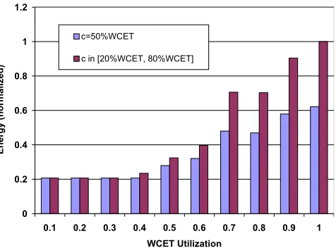
Figure 1.1: Look-ahead RT-DVS Energy for Constant/Fluctuating Workload

The potential to save energy by combining DVS techniques with operating system scheduling has been investigated in previous work. Significant savings have been reported for general-purpose computing systems [13, 16, 30, 40, 52, 69, 55, 15] as well as real-time systems [19, 20, 32, 63, 53, 10, 47, 14, 2, 29]. DVS algorithms for general-purpose systems often use various heuristics to reduce processor voltage or frequency according to the observed system workload [69, 52, 13]. DVS for hard real-time systems, in contrast, requires more subtle control. Timing requirements must be considered by the DVS algorithms to determine the processor frequency.

(15)

worst-case execution time (WCET) of a task to guarantee the schedulability of the system. A safe upper bound on the WCET of a task can be provided through static analysis, dynamic analysis or a combination of both [56, 51, 17, 73, 37, 18, 1, 35, 36, 12, 49, 68]. Prior experiments have shown a wide variation between longest and shortest execution times for many actual applications. For example, actual execution times of real-world embedded tasks are observed to vary by as much as 87% relative to their measured WCET [68]. Budgeting for the WCET may result in excessive energy consumption even though actual utilization is lower than the worst case.

Also, pure DVS techniques do not perform well for dynamic systems where the sys-tem workloads vary significantly. Many of the existing hard real-time DVS schemes are not able to adapt well to dynamically changing workloads. For example, we compared the energy consumption of Look-ahead RT-DVS [53] between a constant workload and a fluctuating workload, as depicted in Figure 1.1. Both workloads contain three periodic tasks defined as T1={3,8}, T2={3,10} and T3={1,14}, where

Ti=_{WCET,Period_} for i= 1...3. The constant workload consists of tasks whose ac-tual execution times (denoted byc) among different jobs are 50% of their WCET. The fluctuating workload consists of tasks with an average execution time of 50% WCET. Their actual execution times fluctuate between 20% and 80% of their WCET (follow-ing variation patterns similar to Figure 7.1, discussed later). Figure 1.1 demonstrates that, in the worst case, Look-ahead RT-DVS degrades up to 40% for the fluctuat-ing workload. More adaptable DVS schemes are required for these workloads with dynamic changing execution times.

1.3 Contributions

In this thesis, we develop and evaluate a novel DVS technique for dynamic work-loads, considering practical design and implementation issues. The novel contribu-tions of this thesis over previous work include:

(16)

achieve better adaptivity for dynamic task sets with fluctuating execution times. The speed of the processor is adjusted dynamically by the operating system. The feedback technique enables the system to select the appropriate frequency and voltage settings so that energy consumption is significantly reduced. It also helps guarantee the timing requirements of hard real-time tasks so that deadlines are not missed. Different feedback control structures are evaluated in our implementation. To the best of our knowledge, this is the first study of feedback control techniques exploiting DVS for hard real-time systems.

• A combined intra-task and inter-task DVS scheme. In contrast to compiler-directed intra-task DVS algorithms where the speed of a task is changed multiple times during program execution, the combined intra-task and inter-task DVS scheme presented in our work divides the execution budget of a task into at most two portions. Keeping the first portion at a low speed makes our algorithm more aggressive than a pure inter-task DVS algorithm. Changing the speed at most once for each task incurs lower overhead than that of a pure intra-task DVS algorithm.

• Slack passing and preemption-handling schemes for DVS schedulers. These schemes ensure the timing requirements of hard real-time tasks. They follow a greedy policy by passing as much slack as possible to scale the next running task. It speculates on the early completion of each task to aggregate unused slack for other tasks. When preemption occurs, the preempted task relinquishes its remaining slack and passes it on to the next task, while reserving enough slack in the future to avoid deadline misses. Different slack reservation schemes are studied to ensure the schedulability of the system.

(17)

other DVS algorithms. The comparison of synchronous and asynchronous DVS switching shows that the energy saving under asynchronous switching is not as significant as expected. The experimental results reveal that the V2_f _power

model (Equation 1.1) works well for DVS performance analysis.

• An extension of the feedback-DVS scheme to embedded architectures where the dynamic power is not dominant. An combined DVS and leakage control scheme is presented to save both static and dynamic power. It automatically alternates between a voltage-scaling mode and a processor sleep mode, according to the execution scenario of tasks. Simulation experiments show that the combined DVS and leakage control scheme saves 15% additional energy on average over a pure sleep policy and 30% additional energy on average over a pure DVS algorithm.

1.4 Dissertation Outline

(18)

Chapter 2 Related Work

The proposed feedback-DVS frame combines feedback real-time control with dy-namic voltage scaling techniques. In this chapter we describe some of the related research work.

2.1 Dynamic Voltage Scaling

Dynamic voltage scaling has been studied by many researchers for general-purpose systems as well as real-time embedded systems. DVS for general-purpose systems is different from DVS for real-time systems. On one hand, general-purpose systems do not need to maintain any workload timing requirements, which have to be guaranteed by real-time systems. On the other hand, general-purpose systems have no knowledge of the system’s worst-case behavior, which is usually available in real-time systems.

A DVS algorithm can be either on-line or off-line. On-line algorithms assign the processor frequency at run-time according to the dynamic state of the system. Off-line algorithms determine the processor frequency statically, before the execution of the system.

(19)

be-ginning of each interval according to the CPU utilization of previous execution traces. Govil et al. compared a number of DVS policies in a simulation environment. Their work suggested that a simple smoothing algorithm was better than a more complex algorithm. Since then, DVS strategies were further evaluated and extended by Pering

et al. [52] and Grunwald et al. [16]. Pering et al. examined DVS algorithms through trace-driven simulation. Grunwald et al. evaluated DVS policies through physical measurements. Chandrasenaet al. [7] incorporated the strengths of the conventional workload averaging technique and the rate selection algorithm. System workloads are buffered to estimate the CPU rate until the scaling factor matches the system quantized rates. Saputra et al. [61] presented off-line compiler-directed DVS algo-rithms based on integer linear programming to accommodate energy and performance constraints.

(20)

decrease significantly. Saewonget al. [60] proposed a series of voltage scaling schemes targeting different hardware configurations and task set characteristics. Their results show that some non-optimal schemes may be more suitable than optimal schemes when the system has a high voltage scaling overhead.

When DVS algorithms are applied to real-time systems, timing requirements of real-time applications pose additional challenges. Lee et al. [33] presented a branch-and-bound algorithm to determine statically the operating frequency of real-time task sets. Due to the complexity of the algorithm, only two frequency levels are assumed in their model. The algorithm proposed by Liu et al. [39] derives optimal speed functions between an upper bound and a lower bound of processor cycles. Their on-line algorithm reclaims unused execution cycles to further reduce energy consumption. Pillai and Shin [53] proposed a set of dynamic DVS algorithms based on traditional hard real-time mechanisms, namely rate-monotone scheduling and earliest-deadline-first scheduling. They extended the schedulability test of RM and EDF algorithms to incorporate CPU frequency scaling. Static DVS, cycle conservative DVS, and look-ahead DVS are presented. Look-look-ahead DVS is the most aggressive DVS scheme among the suite of algorithms proposed. Unlike our algorithm which applies frequency scaling to only the current task, they assumed a unified frequency scaling factor on all tasks. In their most aggressive variant, the look-ahead technique is used to achieve extensive energy savings by deferring as much work as possible. However, the frequency value obtained in their algorithm is not always the lowest possible frequency for a single task, as shown by Dudani et al. [11].

(21)

schedule.

The idea of deriving a feasible dual-level DVS schedule from an ideal case was first proposed by Gruian [14, 15]. It combines off-line and on-line scheduling at both task level and task-set level. Stochastic data derived from previous task execution traces are used to produce energy-efficient schedules. Multiple frequency levels may be assigned to a single task. Our approach, instead, assigns at most two different frequencies for each task. Our algorithm targets dynamic-priority scheduling while Gruian restricts his approach to fixed-priority scheduling. Dual-speed scheduling was also investigated by others. Zhanget al. vary the processor speed between high and low whenever non-preemption blocking occurs [72]. Leeet al. assume an architecture where only two physical speed levels exist [33]. Our approach considers a more gen-eral case where multiple frequency and voltage levels are chosen by subsequent jobs of the same task or even different tasks. Jejurikar and Gupta investigate static and dy-namic slowdown factors for periodic tasks [26] and combine them with procrastination scheduling [27] and preemption threshold scheduling [25]. Several of these algorithms were compared in a unified simulation environment, SimDVS [62]. In contrast, we measure power consumption on a concrete micro-architecture for several EDF-based algorithms.

Last-chance scheduling without energy considerations goes back to Chetto et al.

[8]. We apply their philosophy in a DVS context. We develop a novel DVS variant based on task splitting with exactly two parts. Such a dual-speed approach aggres-sively reduces power consumption if the first subtask is fully utilized while the second subtask never executes. Our feedback approach triggers this behavior, which is supe-rior to Gruian’s step-wise increase of frequencies with a stochastic approach.

2.2 Feedback Real-time Scheduling

(22)

specifications are analyzed systematically through a control-theoretical method. Lu

et al. [42] further proposed a feedback control real-time scheduling framework for un-predictable dynamic real-time systems where task execution times diverge from their worst case . Real-time system performance specifications are analyzed and satisfied systematically through a control-theory based methodology. Dynamic models of real-time systems are developed to identify different categories of real-real-time applications. While their feedback control framework is for general purpose real-time scheduling, our scheme focuses on feedback control schemes for reducing energy consumption of processors.

For multimedia systems, a formal feedback control algorithm combined with dy-namic voltage/frequency scaling technologies was first described by Lu et al. [43]. Both continuous and discrete DVS settings are exploited in their scheme to reduce energy consumption. An adaptive set-point is used to achieve fast responses with a stable multimedia throughput.

(23)

2.3 Leakage-aware DVS Scheduling

Static power consumption caused by leakage current has incurred much attention in recent years. Conventional DVS scheduling strategies are modified to be leakage-aware. Lee et al. [34] proposed greedy methods to maximize the duration of idle and busy periods based on the worst-case execution time [34]. Their algorithms are integrated into conventional dynamic priority scheduling and fixed priority scheduling policies. It is most useful if there are many relatively short inter-task idle periods that can be grouped together. Since actual execution times often diverge considerably from WCET, a conceptual busy period is interspersed with dynamic slack due to early completion of tasks.

Quan et al. described an enhanced DVS algorithm to reduce both dynamic and static power consumption [58]. The latest release time of each job in the task set is computed off-line and subsequently used by an on-line scheduler. Their approach is based on fixed-priority scheduling while ours is based on dynamic-priority scheduling. Their online scheduler always delays the release time of a task to its latest start time (last chance) as long as the processor is idle. Such an aggressive scheme is not always the most energy efficient solution. In our algorithm, we make delay decisions based upon the actual execution time of tasks via feedback, which is more energy efficient on average.

Jejurikarat al. enhanced EDF scheduling with a procrastination algorithm [28]. A delay interval is calculated for each task, which only considers static task information and may result in a pessimistic schedule. Our scheme is integrated with the online scheduler. It converts dynamic slack, generated due to the critical speed threshold or the early completion of tasks, into idle or sleep time. Their approach also assumes that a power manager, implemented as a controller in hardware, handles interrupts and timers when new tasks are released. In contrast, our scheme does not require any special hardware support except for DVS and sleep modes.

(24)

(25)

Chapter 3 Feedback-DVS Framework

In this chapter, we first define the task model used throughout this work. The architecture of the feedback-DVS framework is then described in detail for a better understanding of the scheme.

3.1 Task Model

We use a periodic, fully preemptive and independent real-time task model [38] in our framework. Each task Ti is defined by a triple (Pi, Di, Ci), where Pi is the period of Ti, Di is the relative deadline ofTi, andCi is the worst-case execution time (WCET) of Ti, measured at the maximal processor frequency. We always assume

Di=Pi in our model. The periodically released instances of a task are called jobs.

(26)

EDF Scheduler Voltage/Frequency

Selector Feedback

Controller

−

Actual Execution Time

CA

+

Maximal Schedule

Profile _{Task Queue}

V,f

Figure 3.1: Feedback-DVS Framework

3.2 Architectural Framework

Prior research on DVS for hard real-time system was primarily concerned with guaranteeing the schedulability of the task sets while energy consumption is mini-mized. But in a dynamic real-time environment where the task execution time varies significantly from job to job, a DVS scheduler should be able to adapt to the ever-changing workloads as fast as possible. One important performance metric of such a system is how fast the DVS scheme can adjust the processor speed according to differ-ent workloads so that energy consumption is significantly reduced. To address this is-sue, we propose a framework called feedback dynamic voltage scaling (feedback-DVS). In this framework, we consider the scheduling problem in hard real-time systems with the earliest deadline first (EDF) policy. This framework is based on feedback control that incrementally corrects system behavior to achieve its energy objective, while the hard real-time timing requirements are still preserved. We assume that the processor can operate at several discrete voltage/frequency levels, which reflects contemporary processor technology with support for DVS. When there is no task running on the processor, the processor enters an idle state at a particular voltage/frequency level, usually the lowest voltage/frequency level on that processor.

(27)

of a job and CA

(28)

Chapter 4 Voltage-Frequency Selector

The voltage-frequency selector is responsible for selecting a voltage-frequency pair each time a task is scheduled. Since power consumption increases proportionally to processor frequency and the square of the voltage [24], minimal energy consumption is obtained by running every task at a uniform processor speed. This is only a statically optimal solution. In a dynamic environment where a task’s actual execution time is unknown until the task completes, it is not possible to derive the optimal uniform speed in advance. Our objective is to approximate a close-to-optimal solution by monitoring the actual execution time of each job. The start point of our scheme is the following inequality, which is a modification of the standard EDF [38] schedulability test:

α−1Ck Pk

+ X

i∈{1,...,n}\{k}

Ci

Pi ≤

1 (4.1)

(29)

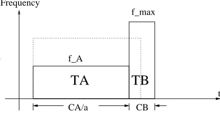
TB

TA

CB

t f_max

Frequency

f_A

CA/a

Figure 4.1: Task Splitting

selector.

4.1 Task Splitting

For each task, the scaling factor α depends on the total available slack when the task is scheduled. For example, at time 0, the available slack for the first task T1

is derived from the expression 4.1 as P1(1−Pni=2

Ci

Pi). Its α value is calculated as:

α = C1

P1(1−Pn_i=2Ci Pi)

. In order to obtain an even lower speed for each task Tk and to make feedback control available for hard real-time systems, our scheme goes beyond that by splitting each task into two subtasks TA and TB. These two subtasks are allowed to execute at different frequency and voltage levels. As shown in Figure 4.1,

(30)

TA or a preemption occurs, the timer can be canceled and no additional overhead will be incurred. Only if execution cannot complete inTA will the timer go off and trigger the DVS operation to enter the TB sub-task.

Let Ck, CA

k and CkB be the worst-case execution cycles of task Tk and its two subtasks, TA and TB. Let sk be the slack available to Tk when Tk is scheduled. We have:

Ck=CkA+C B k ,

CA k

α +C

B

k =Ck+sk (4.2)

we derive α from the above equation:

α= C A k

CA k +sk

(4.3)

Equation 4.3 shows that when task splitting is used, the scaling factor αdepends not only on the amount of available slack (sk), but also on the number of execution cycles assigned to TA. In the following, we describe the methods used to determine these two values.

4.2 Static Slack Utilization

The type of slack available during the scheduling of a real-time system falls into two categories. One is static slack due to under-utilized system workloads. The other one is dynamic slack due to early completion of tasks. In order to exploit these two types of slack, we consider an actual schedule and a maximal schedule. The maximal, schedule, or worst-case schedule, is the schedule produced by a standard EDF algorithm when the execution time of each job equals its WCET. The actual schedule is the actual execution scenario produced by our feedback-DVS algorithm where the execution time of each task varies from job to job. The maximal schedule is constructed offline in O(N) complexity, where N is the total number of jobs executed in a hyperperiod H. The static slack is exploited by adding an idle task,Tn+1, into the

(31)

static slack is not monopolized by a single task but evenly distributed. This also facilitates the online computation of static slack. The idle task has a non-zero WCET but its actual execution time is always zero. The WCET and the period of the idle task are chosen in such a way that the total utilization of the new task set becomes 100%. In other words,

Pn+1 =P1, Cn+1 =Pn+1(1−U), cn+1 = 0. (4.4)

Notice that any other choice of idle task periods is also legal. Most notably, the shortest period of any task, P1, and the longest one, Pn, are interesting choices. We

consider these options since they affect the amount of static slack available for other tasks. We choose the shortest period as the idle task’s period to ensure that there is at least one idle task being released between any task’s invocation to provide static slack for that task. The total static slack generated by idle task Tn+1 in the interval

[t1..t2] is denoted by:

idle(t1...t2) = Σ t1..t2

idle slots (4.5)

4.3 Dynamic Slack Passing

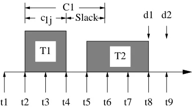
Dynamic slack passing is a technique to reduce the online complexity of slack computation. It is based on the observation that slack generated by one job is usually not exhausted when the job completes. Instead of computing each job’s slack from scratch, the previous job passes its unused amount of slack to the next job. That slack is further augmented by any static idle slots between the deadline of the previous job and the next job.

(32)

c1j

t1 t2 t3 t4 t5 t6 t7 t8 C1

Slack

t9 d1 d2

T1 _T2

Figure 4.2: Dynamic Slack Passing

sij=

   

  

Cp−cpk if rij ≤Ipk +cpk

Fpk−rij if Ipk+cpk < rij< Fpk 0 if rij ≥Fpk

(4.6)

An example is depicted in Figure 4.2. Let task T1 with WCET C1 and deadline

t8 execute its jth _{job with an actual execution time of} _c

1j. Assume that when T1 is

invoked at time t2, it inherits a total slack of S from its previous tasks. T1 is then

scaled to a lower frequency with that slack and completes at time t4. The difference between C1 and c1j is the new slack dynamically generated by T1. So the total slack

available at t5 is S = S +C1 −c1j. Note that the actual execution time c1j may be less than, equal to, or greater than the worst-case execution time C1 because of

task scaling. If C1 > c1j, Equation 4.6 just adds the slack produced by the early completion of T1 into the total slack. If C1 < c1j, Equation 4.6, in fact, reduces the

total slack becausec1j exceeds its WCET in the maximal schedule (it is feasible under DVS as long as the available slack is not exceeded). The adjusted total slack is passed in full or in part to the next task T2 depending on T2’s release time and deadline.

Slack beyond T2’s release time and deadline cannot be used byT2 and, therefore, will

not be passed on to it.

(33)

4.4 Preemption Handling

Preemption handling follows a greedy scheme in that we try to pass as much slack as possible to scale the running task. We speculate on its early completion to aggregate more slack for other tasks. When preemption occurs, the preempted task relinquishes its remaining slack and pass it on to the next task, just as it does when a task completes. But there are two differences here. First, the preempted task itself cannot generate any slack based on its own execution at the preemption point since the task’s completion time is unknown. Hence, no additional slack is added to its inherited total slack. Second, the preempted task still needs some time to complete its execution in the future. The remaining execution time must be reserved in advance to avoid future deadline misses caused by over-exploiting slack from other tasks. At the preemption point, the expected remaining execution time, Lij, of the preempted task is:

Lij =Ci−cij×α−1 (4.7)

wherecij is the actual execution time up to the preemption point. Our slack passing scheme promises that the preempted task will not miss its deadline by reserving the expected remaining execution time from its slack:

sk,r =sk−Lij (future slots) (4.8)

where sk is derived from Equation 4.6 and the resulting slack sk,r is passed to the next task.

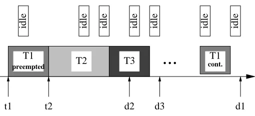
Future slot allocation is essential to ensure the feasibility of the schedule under DVS. Future slots will be allocated only if the maximal schedule does not have suffi-cient slots for the preempted job between the preemption point and the job’s deadline. We devise multiple schemes for reserving these slots.

• Forward sweep: When a task T1 is preempted and requires L1j slots in the future, the preempting task, T2, deducts this amount from its available slack

(34)

...

t1 t2 d2 d3 d1

idle idle idle idle idle idle idle

T2 T3

T1

preempted

T1

cont.

Figure 4.3: Future Slot Reservation

• Backward sweep: Future slots of T1 are allocated from T1’s absolute deadline

d1 backwards. Any of the idle slots in the maximal schedule become unavailable for other tasks, i.e., these slots are excluded in Equation 4.6.

An example is depicted in Figure 4.3. The upper time line of idle slots presents an excerpt of the maximal schedule that depicts idle task allocations. The lower time line shows the dynamic schedule. Upon release of T2 at time t2, T1 is preempted. Let us assume that T1 does not have sufficient static slots (three slots) beyond t2 to finish its execution. It has to rely on future idle slots. During T2’s execution,

T3 is released. Both T2 and T3 have earlier deadlines than T1 (d2 < d3 < d1). Subsequently, T1 only resumes after T3 completes.

Future slot allocation of T1 depends on the chosen scheme. The forward sweep results in zero idle slack for T2 and T3 since idle slots during the tasks’ periods are not sufficient to cover T1’s future execution budget. The backward sweep, on the other hand, reserves the last 3 idle slots from d1 backwards. T2 andT3 have two and one idle slots left, which makes frequency scaling still possible.

Overall, the forward sweep is not as greedy as the backward sweep in the sense that tasks released prior to the preemption point may not be scaled due toT1’s future slots. A forward sweep is likely to result in zero slack for the preempting task T2, if P2 << P1, i.e., the period of T2 is much shorter than T1’s period. Fewer idle

(35)

(36)

Chapter 5 Feedback Controller

This chapter first reviews the basic PID feedback control design. It then presents a single proportional-feedback control design, a multi-input control design, and a single-input control design for our DVS algorithm. Finally, the stability of the feedback-DVS system is analyzed.

5.1 Basic PID Control

Equation 4.3 shows that the scaling factor α of a task Ti depends not only on the amount of available slack but also on CA

i , the number of execution cycles assigned to the first subtask TA. Static slack utilization and dynamic slack passing, as described in the previous chapters, help us determine the amount of slack available for each task. In this section, we focus on another key issue, i.e., how to determine the value of CA

i . Since CiA is based on the estimated worst-case execution time of the first subtask TA, our objective is to let CA

i approximate Tij’s actual execution time cij so thatTij can completes before it enters the second subtaskTB. Most of all, when Tij’s actual execution time cij does not exceed CiA, all of Tij executes at a low frequency corresponding to α. It is not necessary for Tij to switch to the maximum processor frequency. Hence, a near-optimal energy consumption is obtained.

(37)

leading to higher processing demands up to some peak point and receding demands after that point. Past work in dynamic real-time scheduling has demonstrated that adaptive techniques derived from control theory can enhance a schedule by reacting to tendencies in execution time fluctuations [41]. In order to devise a DVS algo-rithm adaptive to such a dynamic environment, we integrate a closed-loop feedback controller into our DVS systems.

Feedback control is one of the fundamental mechanisms for dynamic systems to achieve equilibrium. In a feedback system, some variables, i.e., controlled variables, are monitored and measured by the feedback controller and compared to their desired values, so-called set points. The differences (errors) between the controlled variable and the set point are fed back to the controller repeatedly. Corresponding system states are usually adjusted according to the differences to let the system variables approximate the set points as closely as possible.

PID-feedback control is a continuous feedback controller capable of providing so-phisticated control response. The controlled variable can usually reach its set point and stabilize within a short period. A PID controller consists of three different ele-ments, namely, proportional control, integral control, and derivative control. Propor-tional control influences the speed of the system adapting to errors, which is defined as the difference between the controlled variable and the set point, by a pure propor-tional gain item. Integral control is used to adjust the accuracy of the system through the introduction of an integrator on past error histories. Derivative control usually increases the stability of the system through the introduction of a derivative of the errors.

(38)

output=KP ×i+_K1_I

R

idt+KDd_dti (5.1) where KP, KI and KD are the proportional, integral and derivative parameters, respectively, and (t) is the system error. The transfer function of the PID controller in the Laplace-domain (s-domain) is given by:

GP(s) =KP + K_sI +sKD (5.2)

5.2 Proportional Feedback Control Design

A periodic real-time workload may exhibit a relatively stable behavior during a certain interval of time. Thus, the actual execution time of different jobs remains nearly constant or only varies within a very small range. For such workloads, we use a specific PID feedback controller, which includes only a proportional control element. We choose the value of CA

i as the controlled variable while cij is chosen as the set point. CA

i is chosen as 50% of the WCET for the first job of each task. While half of the task’s execution is budgeted at a low frequency, half of it is reserved at the maximum frequency. The task can still meet its deadline, even if the worst case is exhibited. Initially, the energy consumption may be significant and is likely to differ from the optimal case due to inappropriate estimations of the actual execution time. Over time, we replace CA

i with the actual execution time of the task based on the execution time fed back after each task completion. The average value of execution times over past executions is utilized to anticipate future CA

i portions. On the average, this scheme allows us to complete the entire task’s budget at a low frequency level, which closely approximates the optimal energy-saving schedule. Let

CA

ij be the anticipated worst case execution time of the first sub-task of job Tij. We define the following equations to get CA

i,j+1, the anticipated worst case execution time

of the first sub-task of job Ti,j+1:

CA

i1 = 0.5×W CET

CA

i,j+1= (CijA×(j−1) +cij)/j, j ≥1

(39)

where cij is the actual execution time of the jth job of task Ti. Each time a job completes execution, its actual execution time is fed back and aggregated to anticipate the next job’s actual execution time, which is further used to calculate an ideal scaling factor for that task.

Although such a proportional feedback scheme only considers a pure gain adjust-ment over the anticipated CA

i value, it works well for real-time task sets where each task either has a constant actual execution time or it has an execution time vary-ing within a small bounded range. For task sets with highly fluctuatvary-ing execution times, more sophisticated feedback schemes are required, which is detailed in the next sections.

5.3 Multi-input Control Design

The proportional feedback control described in the previous section follows a pro-portional adjustment relative to average execution times. In practice, real-time em-bedded systems, such as audio and video playback or image processing systems, often experience fluctuating execution times of tasks over a period of time. The fluctua-tions may result in tendencies leading to higher processing demands up to some point and receding demands after this peak point. In order to devise a DVS algorithm adaptive to such a dynamic environment, more sophisticated feedback schemes are needed. According to the objective described above, we design a feedback scheme presented as a multiple-input (MI) control system. For every task Ti in the system, its CA

i value is chosen as the controlled variable while its actual execution time cij is chosen as the set point. The system error is defined as the difference between the controlled variable and the set point, i.e.,

ij=cij−CijA. (5.4)

The error is measured periodically by the controller. Its output is fed back to the feedback-DVS scheduler to adjust the value forCA

i . For ntasks in the task set, there are altogether n feedback inputs (ij, i=1...n ) and n system outputs (CA

(40)

For each task Ti, let CA

ij be the estimated CiA value for its jth job. The following discrete PID control formula is used in our feedback-DVS scheduler:

∆CA

ij =KP ×ij+ _K1

I P

IWij+KD

ij−i(t−DW)

DW

CA

i,j+1 =CijA+ ∆CijA

(5.5)

where KP, KI and KD are proportional, integral, and derivative parameters, respec-tively. ij is the monitored error. The output ∆CijA is fed back to the scheduler and is used to regulate the next anticipated value forCA

i . IW and DW are tunable window sizes such that only the errors from the last IW (DW) task jobs will be considered in the integral (derivative) term. We use DW = 1 to limit the history, which en-sures that multiple feedback corrections do not affect one another. The three control parameters KP, KI and KD adjust the control response amplitude and its dynamic behavior with great versatility. It is therefore important to choose and tune these parameters for the controller. The process of adjusting the control parameters is compromised among different system performance metrics. For example, the system may be tuned to have either a stable but slow control response, or an instable but dynamic control response. What is preferred in our system is a sufficiently rapid and stable control output during the entire scheduling process.

(41)

In order to address the drawbacks brought by the complexity of the MI control system, we transform the above MI model into a single-input (SI) control model in the following.

5.4 Single-input Control Design

We now present a simplified design for the system model. Instead of using CA

i (i = 1...n) as the controlled variable for each task Ti and creating n different feedback controllers for n different tasks, we now define a single variable r as the controlled variable for the entire system as:

rj = 1

n

X

i=1

CA ij −cij

cij

(5.6)

where j is the index of the latest job of taskTi before the sampling point. rj describes the average difference between tasks’ actual execution times and their corresponding

CA

i values. Our objective is to makerapproximate 0 (i.e.,the set point). The system error becomes

(rj) =rj −0. (5.7)

where(rj) reflects the error of the entire task set and is not a function of a particular task Ti anymore. (rj) is further fed back to the PID scheduler to regulate the controlled variable r. The PID feedback controller is now defined as:

∆rj =KP ×(rj) + _K1

I P

IW(rj) +KD

(rj)−(rj−DW)

DW

rj+1 =rj+ ∆rj

(5.8)

where KP,KI and KD are the PID parameters. IW and DW are the integral and derivative window sizes.

(42)

the memory requirement of the system since only one global feedback queue needs to be created instead of n different queues for n different tasks in the multi-input feedback scheme. Such a transformation simplifies the control system so that there is only one system input(t) and one system outputr. It eases the analysis and implementation of the feedback controller in our scheduler. But a drawback of the model is that it does not provide direct feedback of the CA

i value for each individual task. A zero value of r may not necessarily imply that each task Ti’s CA

i has approximated its actual execution time. It is only an imprecise description of the original scheduling objective and may take longer to get the system into a stable status. But we expect that this model still captures the characteristics of the overall system behavior and leads to acceptable performance, which has been confirmed in our experiments. In the following, we analyze the system to assess the stability of our control model.

5.5 Stability Analysis of the Single-input Feedback

Control

Stability is an important metric for real-time control systems. A control system is stable if its controlled variables are always bounded for bounded input performance references and disturbances. In order to analyze the stability of the above single-input control model, we compute its transfer function in the Laplace domain. The transfer function of the PID controller is defined as:

GP ID(s) =KP +

KI

s +KDs (5.9)

The transfer function between rj andCiA can be derived by taking derivative of both sides of the equation 5.6:

Gr(s) = M s (5.10)

where M = 1_nPn

i=1 1

ci. Therefore, the transfer function of the entire closed-loop

(43)

GP ID(s)Gr(s) 1 +GP ID(s)Gr(s) =

M KPs+M KI+M KDs2 1 +M KPs+M KI +M KDs2

(5.11) According to control theory, a system is stable if and only if all the poles (the denominator of its transfer function) are in the negative half-plane of the s-domain. From Equation 5.11, we infer the poles of our system as

−M KP ±√M KP2 −4M KD(M KI+ 1) 2M KD

(44)

Chapter 6 Algorithm and Its Correctness

This chapter presents an algorithmic description of the feedback-DVS scheme in pseudo-code. Some examples are then given to explain the scenario when the algorithm is applied on real-time task sets.

6.1 Algorithm Description

An algorithmic description of our feedback-DVS scheme with the PID feedback control is given in Algorithm 1. The following notations are used in the algorithm description:

• Tij: the j-th job of task Ti

• prev: the index of the previous job immediately scheduled before Tij

• now: the current time

• Pi: the Period of Ti

• dij: the absolute deadline ofTij

• Ci: the WCET ofTi (without scaling)

• CA

i : the anticipated worst-case execution time of the first sub-task (low fre-quency portion) of Ti

• CB

(45)

• cij: the actual execution time of Tij up to now (with scaling)

• KP, KI, KD: the PID parameters

• IW, DW: the integral and derivative window size

• Lij: the worst-case remaining execution time ofTij (without scaling)

• slack: the current slack of the system

• idle(t1..t2): the amount of idle slots between times [t1,t2]

• completed(t1..t2): slots of already completed tasks between times [t1,t2]

• slots(Tij, t1..t2): the amount of time slots reserved for Tij in the worst case between times [t1,t2]

• f: the processor frequency

• fm: the maximal processor frequency

• α: the frequency scaling factor

This algorithm integrates the PID feedback scheme and preemption-handling with future slot reservation. Only the MI control model is presented in the pseudo-code. The SI model is implemented in a similar way. The online complexity of our algorithm is O(n) for n tasks, because the length of slots in the maximal schedule during the interval between the release time and deadline of the current task has to be updated when a task is released or completes. The number of slots in this interval is bounded by the number of tasks because only a constant number of jobs for each task and a constant number of preemptions may occur in this interval.

Next, let us see some examples of applying the algorithm on real-time task sets.

6.2 Examples

(46)

Algorithm 1: Feedback-DVS

Procedure Initialization begin

foreachTk∈ {T1, T2, . . . , Tn}do

CA

k ←Ck/2; Lk0←Ck; ti←0

U ←C1

P1 +

C2

P2 +. . .+

Cn

Pn

Pn+1←P1; Cn+1←P1×(1−U)

cn+1←0; slack←0

end

Procedure TaskActivated (Tij) begin

if processor was idle f or d then slack←slack−d

if Tprev was prempted/interruptedthen Lprev=Cprev−cprev×α0

slack←slack−idle(dij..dprev)

if Lprev> slots(Tprev, now..dprev) then

reserveprev←Lprev−slots(Tprev, now..dprev) allocate reserveprev in [now...dprev]

else

if now > dprev then

slack←slack−idle(dprev, now) slack←slack+idle(dprev..dij) α0 ←min{f1

fm, . . . ,

fm

fm|

fi

fm ≥

CAij

CAij+slack}

if α0= 1 then CA

ij ←0

else CA

ij ←slack×α0/(1−α0) SetInterrupt(Ti, CA

ij/α0)

SetFrequency(α0) end

Procedure Taskcompleted (Tij) begin

slack←slack−cij+Ci ←cij−CA

ij ∆CA

ij ←Kp∗(ti) +1I

P

IW(ti) +D

(ti)−(ti−DW)

DW CA

i,j+1 =CijA+ ∆CijA

ti←ti+ 1; Li(j+1)=Ci

if reserveij >0then release up to |reserveij|

end

Procedure SetInterrupt (Tij, CA

ij)

begin

Set timer interrupt f or Tij at CA

ij time units end

Procedure SetFrequency (α0) begin

(47)

100% 50% 75% 25%

5 10 15 20 25 30

t 0 T1 T2 T3 T1 T2 T1 T3 T2 T1 T2

I I I I I I I

2 idle for T1 1 idle for T2

(i) Static Worst-Case EDF Schedule with Idle Task I 100%

50% 75% 25%

5 10 15 20 25 30

t 0

T2 T1

2 idle _{1 idle}

1 slack

T3 T1 T2 T1.A T1.B T3 T2 T1 T3

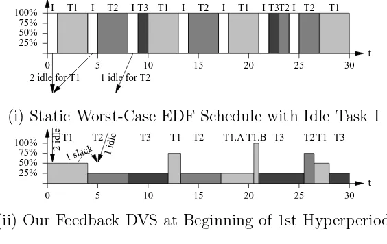
(ii) Our Feedback DVS at Beginning of 1st Hyperperiod Figure 6.1: Discrete Scaling Levels for 3 Tasks

of T1, who has an actual execution time of two. All scheduling events (task release, preemption, resumption, and completion) of the maximal EDF schedule are stored in a look-up table to reduce time complexity.

Next, the task set is scheduled according to our algorithm (without the idle task). Additional operations to calculate slack and to set the CPU frequency/voltage are inserted at scheduling points. As shown in Figure 6.1(ii), when the first taskT1 (with

the earliest deadline) is activated at time 0, its initial slack is assigned according to Equation 4.6. The initial slack s1,0 is set to 0 since no previous task had been

scheduled. The value ofidle(0..d1) is obtained from the pre-calculated maximal EDF

schedule. Then, a frequency scaling factor α is set according to Equation 4.3: α =

CA

k/(CkA+sk). The CPU frequency is set to α∗fm. When the first task completes, unused slack is adjusted and passed on to the next task according to Equations 4.7 and 4.8. The estimated value of CA

1 for the first task is updated according to our

feedback scheme. When the second task is scheduled, its slack is again determined by Equation 4.6, this time with a non-zero slack on the right-hand side of the equation (since the first task passes no unused slack). The frequency level is determined in a similar way as the first task. For later task instances, the feedback scheme chooses

CA

(48)

applied but not shown here to simplify the example.

The effect of the PID feedback scheme is shown in the following example. Consider a task set of three tasks T1=_{12,32_}, T2=_{12,40_} and T3=_{4,65_}. Let the actual execution times of different jobs of a task fluctuate according to the execution time pattern 1, as depicted in Figure 7.1. Figure 6.2(a) is a snapshot of the feedback-DVS schedule for this task set without PID-feedback. Figure 6.2(b) depicts the feedback-DVS schedule for the same task set using feedback with PID parameters CP=0.9, CI=0.08 and CI=0.1.

100%

50% 75%

25%

480 500 520 540

Ca Cb

T1 T2 T1 T3 T2

t

25% 50% 75% 100%

480 500 540

Ca Cb

T1 T2 T1 T2

520 T3

t

(b) DVS−EDF Schedule with PID Feedback (a) DVS−EDF Schedule without PID−Feedback

Figure 6.2: Schedules: Simple and PID Feedback

We can see from the figures that the first job of T3 and the second job of T2 are

scheduled to run at a much lower frequency in the PID feedback schedule than the one without PID-feedback. The first job of T3 with an actual execution time of 2.57

starts at time 524 in the schedule without PID-feedback, while it starts at time 520 in the PID feedback schedule. The PID feedback scheme gets an execution time of 3.06 for its CA

3,1 according to Equation 5. With the closer approximation of c3,1, the

PID scheduler is able to scale the task more aggressively than the one without PID-feedback. Similarly, the non-feedback schedule only gets an average execution time of 5.26 for the second job of T2, which has an actual execution time of 7.07. But

the PID feedback scheme obtains a CA

(49)

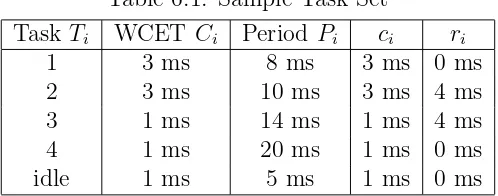
Table 6.1: Sample Task Set

Task Ti WCET Ci PeriodPi ci ri

1 3 ms 8 ms 3 ms 0 ms

2 3 ms 10 ms 3 ms 4 ms

3 1 ms 14 ms 1 ms 4 ms

4 1 ms 20 ms 1 ms 0 ms

idle 1 ms 5 ms 1 ms 0 ms

execution time. This demonstrates the superiority of our feedback-DVS scheme in adapting to dynamic workloads resulting in additional energy savings.

6.3 Correctness of the Algorithm

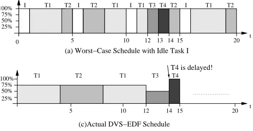
In traditional EDF scheduling, any job’s actual start time si is less than or equal to its worst-case start time in the maximal schedule. But this is no longer the case in our feedback-DVS schedule. Because feedback-DVS may extend a job’s execution time to be longer than its WCET, a job’s actual start time may be later than its start time in the maximal schedule. The next example shows a case where a job’s actual start time exceeds its worst-case start time.

Consider the task set in Table 6.1. Its worst-case schedule with an idle task and its actual schedule under feedback-DVS are shown in Figure 6.3(a) and Figure 6.3(b), respectively. When task T3’s second job starts at time 12 in the actual schedule, its

absolute deadline is at time 18. There is only one idle slot between time 12 and time 18, which scales T3 at a 50% frequency level. Since T3’s actual execution time equals

its worst-case execution time, it runs for 2 time units and ends at time 14 with an actual execution time of 2. When T4 starts execution at time 14, it has been delayed

by one time unit relative to its start time in the worst-case schedule.

We show the correctness of our feedback-DVS algorithm, by the following theorem. Theorem 1. The feedback-DVS algorithm results in a feasible schedule for a set T of tasks with periods equal to their relative deadlines if a feasible schedule exists for

(50)

100% 50% 75% 25% T1 t

0 5 10 12 13 1415 20

T1 T1 T1

T2 T2 T3 T4 T2 T2

I I I I

25% 50% 75% 100%

t

5 10 12 14 15

T1 T2 T1 T3 T4

20

T4 is delayed! (a) Worst−Case Schedule with Idle Task I

(c)Actual DVS−EDF Schedule

Figure 6.3: Delayed Start of Tasks due to Scaling

We call the schedule produced by our feedback-DVS algorithm theactualschedule, where the execution time of a task is variable for different task instances (jobs). We call the schedule under EDF where each task’s actual execution time always equals its WCET themaximalschedule. Letsi ands+i beTi’s absolute start times in the actual and the maximal schedule, respectively. We use the simplified shortcut Ti to denote a certain jth _job _T

ij of task Ti. Similarly, let fi and fi+ be the absolute completion times of Ti in the actual and the maximal schedule, respectively. In order to prove the theorem, we first prove the following lemma:

Lemma 1. The difference between a task’s start time in the actual schedule and the maximal schedule is bounded in feedback-DVS by the following inequation:

si−s+i ≤idle(f

+

i−1, di−1) +

X

Tl∈[fi+−1,di−1];dl>di

Cl (6.1)

where idle(fi+−1, di−1) is the length of all idle slots existing between [fi+−1, di−1] in the

maximal schedule. Cl is the WCET of any task Tl in the maximal schedule with a

priority lower than Ti. fi+−1 and di−1 are the completion time and absolute deadline

of task Ti−1, which is the most recently executed task beforeTi.

Proof of Lemma 1 We will use induction to prove the lemma. First, consider the highest priority taskT1 as the base case. SinceT1 always starts execution immediately

at its release time under both the actual schedule and the maximal schedule, we have,

(51)

di Ih dh f+i t di−1 s+i Ti Preempted

(a) Maximal Schedule

di

Ik+Ik+1+Tk Ih Ip

t Th Ti fi si Ti−1 Preempted

(b) Actual Schedule

Ti ( cont.) Ik

Ti ( cont.) Tk Ik+1 Ip Th

Figure 6.4: Maximal vs. Actual Schedule

Hence, the lemma holds for T1.

Now assume that a certain task Ti satisfies the lemma. We need to show that

Ti+1, the task with the next lower priority thanTi, also satisfies the lemma. We only

need to consider the case wheresi+1 > s+i+1, since this is where feedback-DVS diverges

from conventional EDF. The only reason for Ti+1 to be delayed is that some higher

priority tasks are still running at time s+i+1. Without loss of generality, we assume

that in the maximal schedule there are m (m _≥ 0) idle slots and q (q _≥ 0) lower priority tasks in [f_i+₋₁, di−1], namely, Ik,Ik+1,...,Ik+m−1 and Tk, Tk+1,...,Tk+q−1. Their

WCETs are denoted by Ik, Ik+1,...,Ik+m−1 and Ck, Ck+1,...,Ck+q−1, respectively. We

have Pk+m−1

l=k Il = idle(f

+

i−1, di−1). Let Ih = idle(di−1, dh) and Ip = idle(dh, di). It is also possible that Ti be preempted by a certain higher priority task Th during its execution. Figure 6.4 shows a simplified case where only Ik,Ik+1 and Tk are shown before di−1. Since both Ti−1 and Th have priorities higher than Ti, we havedi ≥di−1

and di ≥ dh. We note that at the time s+i in the maximal schedule, all other tasks with priorities higher than Ti must have completed, and all other lower priority tasks will not be scheduled beforef+

i . Only newly released high priority tasks can execute in [s+_i , f_i+] and may preempt Ti. Since the lemma holds for Ti, we have :

si−s+i ≤ k+m−1

X

l=k

Il+ k+q−1

X

l=k

Cl =idle(fi+−1, di−1) +

X

Tl∈[fi+−1,di−1];dl>di

Cl (6.3)

(52)

because it can always preempt Ti at s+h in the actual case, i.e., sh = s+h. When

Ti is preempted at time sh, the forward slack reservation scheme in feedback-DVS reserves Ci − (sh −si), the worst-case remaining execution time left for Ti, from

Tk, Ik+m−1,...forward. The backward slack reservation scheme reserves the above

amount of time from the Ip, Ih,...,backward. In either case, we denote the total execution time of reserved slots by CR. At time s+_h, the frequency scaling decision is made for Th. The scheduler collects all available idle slots and early completion of low priority task slots in [s+_h, dh] in the maximal schedule excluding any slots re-served for future resumption of preempted tasks. The final amount of slack available for Th equals to

Pk+m−1

i=k+1 Ii +Ih+

Pk+q−1

l=k Cl−CR. Th uses the slack to scale itself to a lower frequency and voltage level. It is equivalent to the transformations that move the non-reserved portion of Ik+1,...,Ik+m−1,Ih and Tl backward and move the corresponding portion of Ti forward. The result is shown in Figure 6.4(b). When

Ti resumes execution, it can be scaled again exploiting slack from the idle slots and early-completed task slots before di. Similar transformations apply when moving Ip backward andTi forward. Tireleases all its unused slack when it completes and passes it on to following tasks.

Except for the idle slots and early completion of lower priority tasks, there are no other cases where Ti will be moved forward and thus be delayed during the above transformations. Hence, the following inequation holds:

fi−fi+ ≤idle(fi+, di)−CR+

X

Tl∈[fi+,di]; dl>di+1

Cl (6.4)

Because di ≥ di−1 and di ≥ dh, the aforementioned transformations never move Ti forward beyond di. Hence, Ti will not miss its deadline after these transformations. If the start time of Ti+1 is delayed in the actual schedule by Ti, we have: si+1 = fi and s+_i₊₁ _≥f_i+. From the above equation we get:

si+1−s+i+1 ≤fi−fi+≤idle(fi+, di) +

X

Tl∈[fi+,di];dl>di+1

Cl (6.5)

Hence, inequation 6.1 also holds for Ti+1, and we proved the lemma.

(53)

the next task Ti+1 will not be delayed for more than the interval of idle(fi+, di) +

P

Tl∈[fi+,di]; dl>di+1Cl. In such a worst case scenario, the feedback-DVS scheduler will

always setTi+1’s speed to maximal so thatTi+1’s actual execution time will not exceed

Ci+1. Since in the maximal schedule we always have:

s+i+1+Ci+1+idle(fi+, di) +

X

Cl ≤di+1 (6.6)

From Inequation 6.5 and 6.6, we derive:

si+1+Ci+1≤s+i+1+Ci+1+idle(fi+, di) +

X

Cl ≤di+1 (6.7)

which shows that Ti+1 meets its deadline. Thus, our feedback-DVS always results in

(54)

Chapter 7 Simulation Experiments

This chapter presents the simulation experiments to evaluate the performance of the feedback-DVS scheme. Some of the experimental results are presented and the algorithmic performance is analyzed.

7.1 Experimental Method

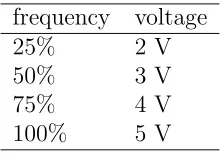
We evaluated the performance of our schemes in a simulation environment that supports feedback-DVS scheduling. In order to make a comparison with our algo-rithm, Pillai and Shin’s Look-ahead RT-DVS algorithm was also implemented [53]. We assume a processor model capable of operating at four different voltage and fre-quency levels, as depicted in Table 7.1. Comparable frefre-quency and voltage settings were also used in the Look-ahead RT-DVS work [53] and the experimental work with StrongARM processors [55]. The results discussed hereafter are also consistent in their trends for power savings on a concrete DVS-capable architecture. In our simu-lations, the processor enters an idle state and operates at the lowest frequency and voltage level when no tasks are ready. We use a simplified energy model in our ex-periment as E =Rt

0 f V2. Energy values reported in the following experiments were

normalized for ease of comparison.

(55)

Table 7.1: Processor Model for Scaling frequency voltage

25% 2 V

50% 3 V

75% 4 V

100% 5 V

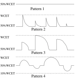
workload patterns. The objective in studying different patterns is to assess the sen-sitivity of feedback DVS to different types of execution time fluctuations, which have been observed in interrupt-driven systems [44]. Since it is not practical to examine every possible type of fluctuation, we constructed three synthesized execution time patterns based on our observation of some typical real-time applications, as shown in Figure 7.1.

(56)

Pattern 2

Pattern 4

Pattern 3

50%WCET

10%WCET 50%WCET WCET

WCET

Pattern 1

50%WCET WCET

(57)

computational needs around peaks. For each execution time pattern, the task sets’ WCETs were uniformly distributed in the range [10,1000]. When tasks’ WCETs were generated, each task’s period was chosen so that the worst case utilization of the task set (i.e., PW CETi

Pi ) varies from 0.1 to 1.0 in increments of 0.1.

Both of the original multi-input (MI) feedback control model and the simpli-fied single-input (SI) feedback control model were evaluated in our experiment. The corresponding feedback-DVS schedulers are referred to as MI Feedback-DVS and SI Feedback-DVS, respectively. Different combinations of PID coefficients were inves-tigated in our experiments. It was observed that both increasing or decreasing the proportional coefficient resulted in less accurate system estimations for CA

i . The derivative item is less significant compared to the other two parameters. Increasing the integral window size improves the energy saving effect in the very beginning, but when IW becomes larger than 10, no dramatic system performance improvements were observed. We restrict ourselves here to report results based on the PID coeffi-cients of KP = 0.9, KI = 0.08, KD = 0.1. The derivative and integral window size were 1 and 10, respectively.

7.2 Results

(58)

!"#$%&'() )!"#$%&'() *%&+'()

Figure 7.2: Execution Time Pattern 1

!"#$%&'() )!"#$%&'() *%&+'()

Dynamic Voltage Scaling with Feedback Scheduling for Real-time Embedded Systems

Biography

Acknowledgements

Contents

List of Figures

List of Tables

Chapter 1

Introduction

1.1