Reduction and normal forms for a delayed reaction–diffusion differential system with B–T singularity

R E S E A R C H

Open Access

Reduction and normal forms for a delayed

reaction–diffusion differential system with

B–T singularity

Longyue Li

_{, Jianzhi Cao}

_{and Yingying Mei}

*_{Correspondence:}

[email protected]

1_{Air and Missile Defense College, Air}

Force Engineering University, Xi’an, China

Full list of author information is available at the end of the article

Abstract

In this paper, we expanded our computation to obtain a simpler and detailed reduction and normal form of a delayed reaction–diffusion differential system with Bogdanov–Takens (B–T) singularity. By using the central manifold reduction method, we try to reduce the dimension of phase space without changing the dynamic behavior of the system. Next, by normal form theory, we try to simplify the form of differential equations, and then succeeded in obtaining a simpler and more specific parameterized delayed ordinary differential system on its center manifold. Finally, two examples show that the given algorithm is effective.

Keywords: Ordinary differential equations; Complex dynamical system; B–T

singularity; Delayed reaction–diffusion differential system; Central manifold reduction

1 Introduction

Common bifurcations include the Hopf bifurcation and the B–T bifurcation, a B–T bifur-cation is a well-studied example of a bifurbifur-cation with co-dimension two, meaning that two parameters must be varied for the bifurcation to occur. It is named after Bogdanov and Takens, who independently and simultaneously described this bifurcation [1–3]. At the Bogdanov–Takens bifurcation, for the system there may appear a saddle node bifurcation, Hopf bifurcation or homoclinic bifurcation, and the B–T bifurcation can further provide more information about periodic behavior and global dynamic behavior. We discuss the bifurcation phenomenon, which is to find the universal unfolding of the system, however, due to the diversity of disturbances, finding a universal unfolding is not easy. Over the past 40 years, great progress has been made in the bifurcation analysis of functional dif-ferential equations [4–10]. Most of the current bifurcation theory studies are focused on ordinary differential systems or delayed differential systems. In real nature, many phenom-ena can be more realistic if they are described by partial functional differential equations, so people pay more and more attention to the application of partial functional differential equations. There are two difficulties in bifurcation analysis for reaction–diffusion systems with time delay. If the system contains both time delay and diffusion, it will become an infinite dimensional dynamic system. The characteristic equation of the linearized equa-tion at a certain equilibrium state is a transcendental algebraic equaequa-tion, and it is difficult to calculate its characteristic root. On the other hand, it is difficult to analyze the

values of infinite dimensional operators, especially in the analysis of the existence of the bifurcation and the stability of its periodic solution.

As is well known, the dimension of an ordinary differential system with B–T singular-ity is at least 2, but this is not true for delayed differential system and reaction–diffusion system. Faria and Magalhães showed that B–T singularity may happen in scalar delayed differential system [4]. Furthermore, in some special cases, reaction–diffusion system can undergo B–T bifurcation only needing one parameter to take its critical value, which sug-gests that reaction–diffusion system can display more complex dynamical behavior [11]. Xu and Huang gave a necessary and sufficient condition to characterize the B–T singu-larity in the first place. Meanwhile, Xu and Huang described the bifurcation behavior of system with B–T singularity in detail [12]. In our previous paper [13], we have studied a class of delayed reaction–diffusion systems,

⎧ ⎪ ⎪ ⎨ ⎪ ⎪ ⎩

ut=Du(x,t) +M(α)u(x,t) +N(α)u(x,t– 1)

+f(u(x,t),u(x,t– 1),α), t≥0,x∈(0,π), ∂u

∂ν = 0, x= 0,π,

(1)

whereα= (α1,α2)∈R2_{is the bifurcation parameter,D=diag(d}

1,d2, . . . ,dn),x∈Ω= (0,π),

u(x,t) :Ω ×R→Rn_{. is the Laplacian operator in R, the homogeneous Neumann}

boundary condition ∂_∂νu= 0 shows that there is no movement on the boundary.

We have already analyzed the generalized eigenvector associated with zero eigenvalue, an equivalent condition for the determination of B–T singularity is obtained. Next, by us-ing center manifold theory and normal form method, we had a two-dimension ordinary differential system on its center manifold. In this paper, we will expand our computation to obtain a simpler and detailed reduction and normal form of system (1). By using the central manifold reduction method and normal form theory, we try to reduce the dimen-sion of phase space without changing the dynamic behavior of the system, and succeeded in obtaining a simpler and more specific parameterized delayed ordinary differential sys-tem on its center manifold. The contribution of this paper and its difference with [13] is that, first, compared with Theorem 2 in [13], Lemma1have defined the basis of,P˜ and its conjugate spaceP˜∗, and determined six conditions for calculating parametersφ0₁,ψ₂0, coefficients ofφ₂0,ψ₁0and coefficients ofφ₁0,ψ₂0, we also completed the detailed proof of Lemma1. Second, we have calculated in detail one basis ofV4

2(R2), their images under

M₂, one basis ofIm(M1

2)c, these are the most critical results in the derivation Theorem1.

Third, by comparing with [13], we find that the delayed reaction–diffusion differential sys-tem and the delayed differential syssys-tem have the same normal form of B–T bifurcation, except atΦ(θ) andΨ(s). For the reduced system (26), its local bifurcation behavior is de-termined by linear and second-order terms, rather than by higher order terms. In (26), we ignore the terms higher than the second-order terms, and give a brief list of the results for sufficiently smallμ1,μ2andε= 1. Thus, Theorem2proposed the phase diagram of the

2 Preliminaries

The first of our basic assumptions on system (1) is:

(H1) M(α),N(α)areCr_{(r≥2) smooth matrix-valued functions fromR}2_toRn×n_,

f(x,y,α)is aCr_{(r≥2) smooth function fromR}n_×Rn_×R2_toRn_{, and}

f(0, 0,α) = 0, ∂f

∂x(0, 0,α) = 0,

∂f

∂y(0, 0,α) = 0, ∀α∈R

2_{, (2)}

d

dαf(0, 0,α) = 0,

d dα

∂f

∂x(0, 0,α) = 0, d dα

∂f

∂y(0, 0,α) = 0,

∀α∈R2.

(3)

LetM=M(0),N=N(0), then (1) becomes ut=Du+Mu(x,t) +N(x,t– 1) +

M(α) –Mu(x,t)

+N(α) –Nu(x,t– 1) +fu(x,t),u(x,t– 1),α. (4)

Cn=C([–1, 0],Rn) is used to represent the space of the continuous mapping from [–1, 0]

toRn_{. Let}

ηα(θ) = ⎧ ⎪ ⎪ ⎨ ⎪ ⎪ ⎩

M(α) +N(α), θ= 0,

N(α), –1 <θ< 0,

0, θ= –1.

Hereηα(θ) is a matrix-valued function with bounded variation on [–1, 0]. Note that

M(α)u(x,t) +N(α)u(x,t– 1) = 0

–1

dηα(θ)u(x,t+θ).

LetV1(t) =u1(·,t),V2(t) =u2(·,t), . . . ,Vn(t) =un(·,t),V= (V1,V2, . . . ,Vn)T, then

L(α)Vt=

0

–1

dηα(θ)ut(θ)

can be regarded as a bounded linear operator fromCntoRn, whereVt(θ) =V(t+θ). If α= 0, then we have

L(0)Vt=

0

–1

dηα(θ)u(t+θ) =MV(t) +NV(t– 1)L0Vt.

According to the definition ofL0, we can getL0(ζ) = (M+N)ζ,L0(θ ζ) = –Nζ,L0(θ2ζ) =

Nζ,∀ζ∈Rn, andL0(eλθζ) = (M+Ne–λ)ζ,∀ζ ∈Rn. System (1) becomes ˙

V(t) =DV(t) +L(α)Vt+f(Vt,α), (5)

(4) becomes

˙

V(t) =DV(t) +L0Vt+ L(α)Vt–L0Vt+Ff(Vt,α)

Linearize (6) at (Vt,α) = (0, 0), then [14,15]

˙

V(t) =DV(t) +L0Vt. (7)

The solution of (7) defines aC0semigroup{T0(t) :t≥0}onCn, its infinitesimal

gener-atorA0:Cn→Cncan be defined as

A0φ=φ˙,

D(A0) =

φ∈Cn:φ˙∈Cn,φ(0) =D(),φ˙(0) =Dφ(0) +L0φ

,

(8)

(7) is equivalent to

˙

V=A0V.

We know that the spectrum ofA0is only a point spectrum, that is,σ(A0) =σp(A0), and

λ∈σp(A0) ⇔ ∃y∈dom()\{0}, s.t.λy–Dy–L0

eλ·y= 0. (9)

Under the Neumann boundary condition, the characteristic root ofis –k2 _{and the}

characteristic function isγk=cos(kx),k= 0, 1, 2, . . . . Let

ηk_α(θ) = ⎧ ⎪ ⎪ ⎨ ⎪ ⎪ ⎩

–Dk2_{+M(α) +N(α), θ= 0,}

N(α), –1 <θ< 0,

0, θ= –1.

Thenηk_α(θ) is actually a bounded variation matrix-valued function on [–1, 0], and

–Dk2φ(0) +L(α)(φ) = 0

–1

d ηk_α(θ)φ(θ), φ∈C[–1, 0],Rn.

The further hypotheses of system (1) are: (H2) Ifλ∈σp(A0)\{0}, thenReλ= 0;

(H3) λ= 0is an eigenvalue ofA0with algebraic multiplicity 2 and geometric

multiplicity 1.

If conditions (H1)–(H3) can be satisfied, we say that system (1) has a B–T singularity, (V,α) = (0, 0) is the B–T point. Theorem 1 in [13] gave an equivalent description for B– T singularity in (1), which can be used as a feasible algorithm for determining the B–T singularity.

3 Reduction and normal forms for system (1)

In this section, we will continue to explore the reduction and normal forms for system (1) with B–T singularity, based on the theory in [4,16], we find that (1) can be reduced to a simple two-dimensional ordinary differential system on its central manifold. By (6), we can transform the system (1) with parameters into the following system without parameters:

⎧ ⎨ ⎩

˙

V(t) =DV(t) +L0Vt+ [L(α)Vt–L0Vt+f(Vt,α)],

˙

α(t) = 0. (10)

˜

LetV˜(t) = (V(t),α(t))∈Rn_×R2_{be the solution of (9), then (9) becomes} ˙˜

V(t) =D˜ ˜V(t) +L˜0V˜t+f˜(V˜t), (11)

whereD˜ =diag(D, 02),L˜0V˜t= (L0Vt, 0) is a bounded linear operator fromC˜n+2to Rn×

R2_{. f}˜_(V˜

t) = [L(α(0)) –L0]Vt +f(Vt,α(0), 0) := (fˆ(Vt,α), 0), where Vt ∈ Cn, α ∈ C2 :=

C([–1, 0],R2_).

Consider the linearized system of (11) atV˜t= 0

˙˜

V(t) =D˜ ˜V(t) +L˜0V˜t, (12)

usingA˜0to represent the infinitesimal generator ofC0-semigroup associated with (12),

thenA˜0= (A0, 0). The characteristic roots ofA˜0 include not only all the characteristic

roots ofA˜0, but also two zero eigenvalues whenα˙= 0. LetΓ˜ be the set of all zero

eigen-values (multiplicity computation). Now we consider the decomposition of the phase space Cnof (6). LetCn=P⊕Q, wherePis the invariant space ofA0associated with zero

eigen-values,Qis the complementary space ofP.C∗_n=C([0, 1],Rn∗_{) denotes the conjugate space}

ofCn, whereRn∗ is a n-dimensional row vector space. The conjugate inner product on

C_n∗×Cnis defined as

(ψ,φ) =ψ(0)φ(0) – 0

–1

θ

0

ψ(ξ–θ)d ηk0 0 (θ)

φ(ξ)dξ. (13)

LetΦ(θ) = (φ1(θ),φ2(θ)), (–1≤θ≤0) andΨ(s) =col(ψ1(s),ψ2(s)), (0≤s≤1) denote the

basis ofPand its conjugate spaceP∗, respectively, and satisfy (Ψ,Φ) =I2, where (Ψ,Φ) :=

(ψj,φi),i,j= 1, 2. SinceQ={φ∈Cn|(Ψ,φ) = 0}, we can obtain the following lemma.

Lemma 1 The basis of P and its conjugate space P∗are as follows:

P=spanΦ, Φ(θ) =φ1(θ),φ2(θ)

, –1≤θ≤0,

P∗=spanΨ, Ψ(s) =colψ1(s),ψ2(s)

, 0≤s≤1,

(14)

whereφ1(θ) =φ10∈Rn\ {0},φ2(θ) =φ20+φ10θ,φ20∈Rn, ψ2(s) =ψ20∈Rn∗\ {0},ψ1(s) = ψ₁0–sψ₂0,ψ₁0∈Rn∗,and there is k0∈0, 1, 2, . . .satisfy

(i) –Dk2₀+M+Nφ₁0= 0, (ii) –Dk₀2+M+Nφ₂0= (N+I)φ₁0,

(iii) ψ₂0–Dk₀2+M+N= 0, (iv) ψ₁0–Dk2₀+M+N=ψ₂0(N+I),

(v) ψ₂0φ₂0–1 2ψ

0

2Nφ01+ψ20Nφ02= 1,

(vi) ψ₁0φ₂0–1 2ψ

0

1Nφ10+ψ10Nφ20+

1 6ψ

0 2Nφ10–

1 2ψ

0

2Nφ20= 0.

(15)

Proof By the proof of Theorem 1 in [13], we know that φ1(θ) =φ10∈Rn\ {0},φ2(θ) = φ₂0+φ₁0θ,φ₂0∈Rn_{, and conditions (i), (ii) in (15) hold. Next, the conjugate operatorA}∗

0:

C_n∗→C_n∗ofA0is written as

A∗₀ψ= –ψ˙,

DA∗

0

=ψ∈C1[0,r],Rn∗:ψ(0)∈D(), –ψ˙(0) =Dψ(0) +L∗₀ψ,

(16)

whereL∗₀:C_n∗→Rn∗_{is the formally adjoint operator ofL}

0; we letη0∗(θ) denote the adjoint

ofη0(θ), then

L∗₀(ψ) = 0

–1

ψ(–θ)d η₀∗(θ).

Notice thatA∗₀ψ2= 0 is equivalent to

⎧ ⎨ ⎩

–ψ˙2(s) = 0, 0 <s≤1,

Dψ2(0) +

0

–1ψ2(–θ)d[η∗0(θ)] = 0, s= 0.

(17)

Equation (17) holds if and only if

ψ2(s) =ψ20∈Rn∗\{0}.

There existsk0∈0, 1, 2· · ·which satisfies

–Dk2₀ψ₂0+ψ₂0(M+N) =ψ₂0–Dk₀2+M+N= 0. (18)

Notice thatA∗₀ψ1=ψ2is equivalent to

⎧ ⎨ ⎩

–ψ˙1(s) =ψ20, 0 <s≤1,

Dψ1(0) +

0

–1ψ1(–θ)d[η0∗(θ)] =ψ20, s= 0.

(19)

So we haveψ1(s) =ψ10–sψ20,ψ10∈Rn∗, there existsk0∈0, 1, 2, . . . which satisfies

–Dk2₀ψ₁0+ψ₁0M+ψ₁0–ψ₂0N=ψ₂0,

that is,

ψ₁0–Dk₀2+M+N=ψ₂0(N+I). (20)

So (iii) and (iv) in (15) hold. Finally, by the definition ofΦ(θ) andΨ(s), we have

(ψ1,φ1) =ψ10φ10–

1 2ψ

0

2Nφ01–ψ10Nφ10= 1,

(ψ2,φ2) =ψ20φ20–

1 2ψ

0

2Nφ01+ψ20Nφ02= 1,

(ψ1,φ2) =ψ10φ20–

1 2ψ

0

1Nφ01+ψ10Nφ02+

1 6ψ

0 2Nφ10–

1 2ψ

0

2Nφ02= 0,

(ψ2,φ1) =ψ20φ10+ψ20Nφ10= 0.

In fact, by (i) and (ii) in (15), we know that the fourth equation in (21) hold. The first equation in (21) is equivalent to the second equation, so we can choose an appropriate coefficient forφ₁0,ψ₂0so that all equations of (21) hold, thus, we have completed the proof

of Lemma1.

It is easy to see thatΦ(θ) satisfyΦ˙=ΦJ, whereJ=0 1_{0 0}.

Now we consider the decompositionC˜n+2=P˜⊕ ˜Q, whereP˜ =P×R2is the invariant

space ofA˜0 associated with Γ˜,Q˜ =Q×R,R={v∈C2|v(0) = 0}. The basis ofP˜ and

its conjugate spaceP˜∗are composed of column vectors ofΦ˜ =Φ_{0 I}0

2

and row vectors of

˜ Ψ =Ψ_0I0

2

, and satisfies (Ψ˜,Φ˜) =I4,Φ˙˜=Φ˜J, where˜ ˜J=diag(J, 02).

The central manifold of the delayed reaction–diffusion delayed differential system near the origin can be expressed as (y(x,α),w(x,α)) :R2_×R2_{→ ˜Q=Q×W, wherey(x,α) and}

w(x,α) satisfyy(0, 0) =w(0, 0) = 0,Dy(0, 0) =Dw(0, 0) = 0, respectively. Based on the theory of [4,16], for the fixedα, considering the normal form of (5), we can define the expanded phase space ofCnas follows:

BCn=

φ|φ: [–1, 0]→Rn,

φis uniformly continuous on [–1, 0) and may not be continuous at 0.

BCnis isomorphic toCn×Rn.

Similarly, considering the normal form of (9), we extendC˜n+2toBC˜n+2=BCn×BC2, and

we see thatBC˜n+2is isomorphic toC˜n+2×Rn+2. LetX0andY0denote the matrix-valued

functions on (–1, 0], where

X0(θ) =

⎧ ⎨ ⎩

0, –1≤θ< 0,

In, θ= 0,

Y0(θ) =

⎧ ⎨ ⎩

0, –1≤θ< 0,

I2, θ= 0.

Define

π:BCn→P, π(φ+X0ξ) =Φ (Ψ,φ) +Ψ(0)ξ

,

whereφ∈Cn,ξ∈Rn. Define

˜

π:BC˜n+2→ ˜P,

˜

π(φ+X0ξ,ψ+Y0μ) =Φ˜

˜ Ψ,

φ

ψ

+Ψ˜(0)

ξ

μ

=π(φ+X0ξ),ψ(0) +μ

,

whereφ∈Cn,ψ∈C2,ξ∈Rn,μ∈R2. SinceBC˜n+2=P˜⊕Kerπ˜, we can decompose

Vt αt

=

Φ 0 0 I2

x(t)

α(t)

+

y(t) w(t)

where (x(t),α(t))∈Rn+2_{, (y,w)∈Kerπ˜, then}

Define the operatorM1

mapping fromV4

2(R2) toIm(M12).

According to the hypothesis (H2), we can prove that, for anyμ∈σ(A˜0)\ ˜Γ andq∈N40,

(q,λ˜)=μhold, whereλ˜ = (0, 0, 0, 0) is a vector consisting of elements inΓ˜ (calculated multiplicity). That is to say, (11) satisfies the nonresonant condition with respect toΓ˜. From (24), we know that the normal form of (11) on the central manifold can be written as

Their images underM2are

Usingφjito represent theith element ofφj, we obtain

η2= 2ψ10 n

i=1

(Ei+Fi+Gi)φ10φ10i

+ψ₂0

_n

i=1

(Ei+Fi+Gi)

φ0₂φ₁0_i+φ0₁φ0_2i–

n

i=1

(Ei+ 2Gi)φ10φ10i

.

By comparing with [13], we find that the delayed reaction–diffusion differential system and the delayed differential system have the same normal form of B–T bifurcation, except atΦ(θ) andΨ(s). For the reduced system (26), its local bifurcation behavior is determined by linear and second-order terms, rather than by higher order terms [17]. In (26), we ignore the terms higher than the second-order terms, and letμ1= –

η4₂

4η4₁ρ

2

1,μ2=|ηη21|(ρ2–

η2 2η1ρ1), ε=±1, then (26) becomes

⎧ ⎨ ⎩

˙

x1=x2, ˙

x2=μ1+μ2x2+x21+εx1x2.

(27)

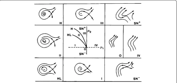
The bifurcation diagram of system (26) can be found in many thesis, such as [17–19]. Here, we give a brief list of the results for sufficiently smallμ1,μ2andε= 1.

Theorem 2 The phase diagram of the system(27)is shown in Fig.1.On the parameter plane(μ1,μ2),we have the following boundary lines:

SN+=(μ1,μ2)|μ1= 0,μ2> 0,

SN–=(μ1,μ2)|μ1= 0,μ2< 0,

H=(μ1,μ2)|μ1= –μ22,μ2> 0

,

HL=

(μ1,μ2)|μ1= –

49 25μ

2 2+o

|μ2| 5 2_,μ

2> 0

.

These boundaries divide the plane into several regions.When(μ1,μ2)is inside these

re-gions,the phase diagram of the system(27)remains unchanged under small perturbations, and the system structure is stable.When(μ1,μ2)is on the boundaries,the system structure

is unstable.Boundary SN+or SN–corresponds to the saddle bifurcations in equilibrium, boundary H corresponds to the Hopf bifurcations,and boundary HL corresponds to homo-clinic orbits bifurcations.

4 Two examples

Example1 Consider the following two-dimensional delayed reaction–diffusion differen-tial system:

First, in order to verify the condition (H2), we will show that the characteristic equation of system (28) has no pure imaginary roots, that is

detλI2+Dk2I2–M–Ne–λ thus (H2) is satisfied.

Now we will verify conditions (i)–(iii) of Theorem 1 in [13]. (1) Fork0= 1,(–Dk02+M+N) =

Example2 Consider the following two-dimensional delayed reaction–diffusion differen-tial system:

ut=Du(x,t) +M(α)u(x,t) +N(α)u(x,t– 1) +f

u(x,t),u(x,t– 1),α, (29)

where D =1 0_{0 1}, M = _α3 1

12+α2

, N =1+α1 1 0 –1+α2

, f(u(x,t),u(x,t – 1),α) = –[u2 1(x,t),

4u22(x,t– 1)]T.

From the discussion of Example1, we know that system (28) has a B–T singularity at (V,α) = (0, 0). Let

ˆ

fu(x,t),u(x,t– 1),α=M(α) –M(0)u(x,t) +N(α) –N(0)u(x,t– 1)

+fu(x,t),u(x,t– 1),α,

its expansion form is

ˆ

fu(x,t),u(x,t– 1),α

=1 2fˆ2

u(x,t),u(x,t– 1),α+h.o.t.

=M1α1u(x,t) +M2α2u(x,t) –N1α1u(x,t– 1) +N2α2u(x,t– 1)

+F1u1(x,t)u(x,t) +G2u2(x,t– 1)u(x,t– 1) +h.o.t., (30)

whereM1=

_{0 0}

1 0

,M1=N2

_{0 0}

0 1

,N1=

_{1 0}

0 0

,F1=

_{–1 0}

0 0

,G2=

_{0 0}

0 –4

.

According to Lemma1, we choose the basis functionsΦ(θ) andΨ(s), where

φ0₁=

1 3, –

1 2

T

, φ₂0=

1 18, 0

T

, ψ₂0= (0, –4), ψ₁0=

0, –4 3

.

By Theorem1, the system (30) can be reduced to ⎧

⎨ ⎩

˙

x1=x2, ˙

x2= (–4₃α1+ 2α2)x1+ (–2₃α1–4₃α2)x2+ 4x12–163x1x2.

(31)

Then (31) becomes ⎧

⎨ ⎩

˙

x1=x2, ˙

x2= –64₈₁(–4₃α1+ 2α2)2–56₂₇α1x2+x21–x1x2.

(32)

5 Conclusions

system with dimension two on its center manifold. Although we have theoretically proved that the system (1) can undergo a B–T bifurcation, unfortunately, due to the limited abil-ity of our computer, it is difficult to display the simulation. For future work, we will firstly improve the ability of our computer and try to display the simulation. Secondly we will not only introduce delays in this model, but also we will study its impact on the analysis of dynamic stability, that is, we will consider executing some control by changing the value of the time delays determined by the system parameters to keep the ecological balance.

Acknowledgements

Not applicable.

Funding

This work was supported by the National Natural Science Foundation of China (No: 71701209, 11771115), Natural Science Foundation of Shaanxi Province of China (No: 2019JQ-250).

Availability of data and materials

The datasets used or analyzed during the current study are available from the corresponding author on reasonable request.

Competing interests

The authors declare that they have no competing interests.

Authors’ contributions

LL developed the idea for the study and wrote the paper; JC and YM did the analyses; all authors discussed the results and revised the paper.

Authors’ information

Longyue Li, Air and Missile Defense College, Air Force Engineering University, No. 1, Changle East Road, Baqiao District, Xi’an, Shaanxi, China;[email protected]. Jianzhi Cao, College of Mathematics and Information Science, Hebei University, Baoding, 071002, China;[email protected]. Yingying Mei, School of Mathematical Sciences, Beijing Normal University, Beijing, 100875, China; Mathematics Group, Xi’an Tieyi High School, Xi’an, 710038, China;[email protected].

Author details

1_{Air and Missile Defense College, Air Force Engineering University, Xi’an, China.}2_{College of Mathematics and Information}

Science, Hebei University, Baoding, China.3_{School of Mathematical Sciences, Beijing Normal University, Beijing, China.} 4_{Mathematics Group, Xi’an Tieyi High School, Xi’an, China.}

Publisher’s Note

Springer Nature remains neutral with regard to jurisdictional claims in published maps and institutional affiliations.

Received: 24 July 2018 Accepted: 7 May 2019

References

1. Bogdanov, R.: Bifurcations of a limit cycle of a certain family of vector fields on the plane. Tr. Semin. Im. I.G. Petrovskogo2, 23–35 (1976)

2. Bogdanov, R.: The versal deformation of a singular point of a vector field on the plane in the case of zero eigenvalues. Tr. Semin. Im. I.G. Petrovskogo2, 37–65 (1976)

3. Takens, F.: Forced oscillations and bifurcations. Commun. Math. Inst. Rijksuniversiteit Utrecht3, 1–61 (1974) 4. Faria, T., Magalhães, L.T.: Normal forms for retarded functional differential equations with parameters and applications

to Hopf bifurcation. J. Differ. Equ.122, 181–200 (1995)

5. Wu, J.: Theory and Applications of Partial Fuctional Differential Equations. Springer, New York (1996)

6. Engelborghs, K., Roose, D., Luzyanina, T.: Bifurcation analysis of periodic solutions of neural functional differential equations: a case study. Int. J. Bifurc. Chaos8, 1889–1905 (1998)

7. Liao, M.X., Tang, X.H., Xu, C.J.: Stability and instability analysis for a ratio-dependent predator–prey system with diffusion effect. Nonlinear Anal., Real World Appl.12, 1616–1626 (2011)

8. Liu, Y., Liu, X., Li, S., Wang, R., Liu, Z.: The Bogdanov–Takens bifurcation study of 2m, coupled neurons system with 2m+ 1 delays. Adv. Differ. Equ.2015, 334 (2015)

9. Li, N.N.: Diffusive induced global dynamics and bifurcation in a predator–prey system. Adv. Differ. Equ.2017, 323 (2017)

10. Xu, R., Gan, Q.T., Ma, Z.E.: Stability and bifurcation analysis on a ratio-dependent predator–prey model with time delay. J. Comput. Appl. Math.230, 187–203 (2009)

11. Faria, T.: Bifurcation aspects for some delayed population models with diffusion. In: Differential Equations with Applications to Biology, pp. 143–158 (1998)

13. Cao, J.Z., Wang, P.G., Yuan, R., Mei, Y.Y.: Bogdanov–Takens bifurcation of a class of delayed reaction–diffusion system. Int. J. Bifurc. Chaos25, 1550082 (2015)

14. Hale, J.K., Lunel, S.M.: Introduction to Functional Differential Equations. Springer, New York (1993) 15. Hale, J.K.: Theory of Functional Differential Equations. Spring, New York (1977)

16. Faria, T., Magalhães, L.T.: Normal forms for retarded functional differential equations and applications to Bogdanov–Takens singularity. J. Differ. Equ.122, 201–224 (1995)

17. Guckenheimer, J., Holmes, P.: Nonlinear Oscillations Dynamical Systems and Bifurcation of Vector Fields. Springer, New York (1983)

18. Chow, S., Li, C., Wang, D.: Normal Forms and Bifurcation of Planar Vector Fields. Cambridge University Press, Cambridge (2004)