R E S E A R C H
Open Access
On the maximum likelihood estimation of the
ToA under an imperfect path loss exponent
Isabel Valera
1*, Bamrung Tau Sieskul
2and Joaquín Míguez
1Abstract
We investigate the estimation of the time of arrival (ToA) of a radio signal transmitted over a flat-fading channel. The path attenuation is assumed to depend only on the transmitter-receiver distance and the path loss exponent (PLE) which, in turn, depends on the physical environment. All previous approaches to the problem either assume that the PLE is perfectly known or rely on estimators of the ToA which do not depend on the PLE. In this paper, we introduce a novel analysis of the performance of the maximum likelihood (ML) estimator of the ToA under an imperfect
knowledge of the PLE. Specifically, we carry out a Taylor series expansion that approximates the bias and the root mean square error of the ML estimator in closed form as a function of the PLE error. The analysis is first carried out for a path loss model in which the received signal gain depends only on the PLE and the transmitter-receiver distance. Then, we extend the obtained results to account also for shadow fading scenarios. Our computer simulations show that this approximate analysis is accurate when the signal-to-noise ratio (SNR) of the received signal is medium to high. A simple Monte Carlo method based on the analysis is also proposed. This technique is computationally efficient and yields a better approximation of the ML estimator in the low SNR region. The obtained analytical (and Monte Carlo) approximations can be useful at the design stage of wireless communication and localization systems.
Keywords: Time-of-arrival estimation, Maximum likelihood estimator, Path loss exponent
1 Introduction
The estimation of a signal time of arrival (ToA), also called time delay, plays an important role in applied sig-nal processing problems, e.g., synchronization [1], array processing [2], tracking and positioning of mobile termi-nals [3-8], or even bioengineering [9]. Let us focus on the estimation of the ToA in wireless radio links. In [10], two simple (and practically appealing) estimators of the ToA are studied: the maximum correlation (MC) and the maximum likelihood (ML) estimators. The MC estimator of the ToA depends only on the correlation between the transmitted and the received signals. The ML estimator of the ToA, on the other hand, takes also into account the path attenuation, which depends on the distance between the transmitter and the receiver, and the path loss expo-nent (PLE) of the environment. The performances of both estimators in mobile positioning applications are analyzed in [8], where it is shown that the ML estimator attains a
*Correspondence: [email protected]
1Department of Signal Theory and Communications, University Carlos III of Madrid, Madrid, Spain
Full list of author information is available at the end of the article
better accuracy when the PLE is perfectly knowna priori. However, the latter assumption is often unrealistic for a practical scenario, because the PLE may change accord-ing to variations in the environment and thus may need to be estimated. Tracking the fluctuations of the PLE is specially important in problems that involve the localiza-tion of mobile terminals, since the existing posilocaliza-tioning techniques based on the ToA estimation are extremely sensitive to errors in the PLE [6].
The problem of dealing with unknown PLEs has been addressed in several related works. In [7], a positioning application with several receivers and one transmitter is considered. The PLEs are assumed to be different and random, with either uniform or normal distributions. The availability of different PLEs for each link increases the localization accuracy compared to the identical PLE assumption. In [11,12], the PLE is estimated from the measurements, whereas in [13-15], several algorithms for the PLE estimation are proposed. The authors of [14] describe three distributed algorithms for PLE estimation in large wireless networks in the presence of node loca-tion uncertainties,m-Nakagami fading and interference.
In [13] and [15], the algorithms for the estimation of the path loss inside a sensor network are designed using previ-ous path loss measurements among sensors. Specifically, in [15], the PLEs are estimated for each node applying the ML criterion and using both ToA and received-signal-strength measurements among the sensors. In [16], a handover algorithm is presented using the least squares estimate of the path loss parameters for each link from a mobile station to a base station. In [17,18], the sensitivity of the ML estimator of the direction of arrival (DoA) of a received signal under model error, i.e., with a mismatch in the PLE, is investigated. To our best knowledge, the prob-lem of estimating the ToA with both the path attenuation and the PLE unknown has not been tackled yet.
The goal of this paper is to investigate the performance of the ML estimator of the ToA under an imperfect PLE. Specifically, we aim at obtaining analytical or semianalyt-ical approximations of the bias and the mean square error (MSE) of the ML estimator, both given in terms of the PLE error and the signal-to-noise ratio (SNR) of the com-munication channel. Such approximations are intended to be useful in the design and setup of the communication and localization wireless systems, as they may consider-ably alleviate the need for a lengthy and computationally expensive simulation of the whole system.
This article is organized as follows. We first describes the signal model and then briefly reviews the expressions of the MC and the ML estimators of the ToA with per-fect knowledge of the PLE in Section 2, including formulas for their MSE performances. In Section 3, we carry out an approximate analysis of the bias and the MSE attained by the ML estimator of the ToA under imperfect PLE. We first apply the method in [18] to study the error between the ML joint estimator of the PLE and the ToA, on one hand, and the ML estimator of the ToA under an imper-fect knowledge of the PLE, on the other hand. The diffi-culty of this study is that the resulting error depends on the ML joint estimates of the ToA and the PLE, which are random variables related to the noise. In order to tackle this limitation and provide an analytical (albeit approxi-mate) expression for the error between the true and the estimated ToA, we analyze the ML estimator of the ToA with mismatched PLE in the second part of Section 3. In particular, we propose a new method to analyze the estimation error based on the Taylor series expansion. In Section 4, we investigate the extension of these results to shadow fading environments [19]. In particular, we first show that the approximate bias is insensitive to the shadow fading, whereas the MSE becomes a random vari-able (the probability density function (pdf ) of which is obtained). Then, we provide a straightforward algorithm to obtain a Monte Carlo estimate of the MSE by draw-ing only from simple Gaussian distributions (instead of simulating the whole transmission system). In Section 5,
we present illustrative computer simulation results based on the transmission of an ultra-wideband (UWB) signal. We have chosen UWB signaling to validate our analysis because it provides an excellent means for wireless posi-tioning due to its high resolution in the time domain [4]. Finally, Section 6 is devoted to the conclusions.
2 Signal model
2.1 Received signal
Consider a wireless transmission link with one single transmitter and one single receiver. Following [20], the received signal can be expressed as
r(t)=as(t−τ )+n(t), (1)
wherer(t)is the received signal,s(t)is the transmitted sig-nal, which is assumed deterministic and possibly complex-valued, a ∈ R+ andτ ≥ 0 are the path gain and the propagation delay (commonly referred to as ToA) between the transmitter and the receiver, andn(t)is the additive noise at the receiver, assumed to be a circularly-symmetric complex-valued zero-mean white Gaussian process with double-sided power spectral density σn2. In (1),τ is the parameter to be estimated.
Assume that the received signalr(t)is observed in the interval(0,To], and letEs =
T0
0 |s(t)|2dtbe the energy
of the transmitted signal in that period. Then, the relation between the transmitted and the received signal energies in terms of the path gain can be written as
Er=a2Es. (2)
In the literature, the path gain a is often modeled as a deterministic parameter (see, e.g., [21-29]). However, it can be elaborated in a more precise way to include the propagation effect [8,10]. In this paper, we assume a com-bined path loss and log-normal shadowing model. The received power in dB is given by (see, e.g., [19], p. 45)
Pr(dB)=Pt+10 log10(κ)−10γlog10(d/d0)−ψdB, (3)
wherePtis the transmitted power in dB,d0is the
close-in distance close-in the far-field region;d = cτ is the distance between the transmitter and the receiver (cis the speed of light),γ is the PLE at the base station,ψdBis a
Gaus-sian random variable with zero mean and variance σdB2 which characterizes the shadow fading (see, e.g., [19], p. 45 and [30], p. 139), andκ is a unitless constant depending on the antenna characteristics and the average channel attenuation given by
κ= c
2
16π2d2 0f02
withf0being the central frequency of the transmitted
sig-nal. If we convert the power in Equation (3) into natural units, then the received energy can also be written as
Er=Es κ ψ
d0
d γ
, (5)
where the random factorψ =10ψ10dB is due to the shadow
fading. Substituting (2) into (5), we obtain an explicit expression for the path gainaas
a= κ
ψ
d0
cτ 1
2γ
. (6)
Let us remark that, since the shadow fading termψdBis normally distributed, the path gainaof Equation (6) is a random variable. For the sake of simplicity, in the analysis of the ML estimator performance in Section 3, we ignore the effect of the shadow fading by taking the expectation with respect to (w.r.t.)ψ ofPr in (3). As a consequence,
the path gain becomes deterministic and reduces to
a=√κ
d0
cτ 1
2γ
, (7)
which coincides with the expression of the path gain already used in [8,10]. The shadow fading effect is taken explicitly into account in Section 4.
2.2 MC and ML estimators of the ToA
In this subsection, we briefly review the MC and ML esti-mators of the ToA. In the literature, the PLEγ is assumed known, and the effect of the shadow fading is ignored; hence, the path gain is deterministic, known and given by (7) [10].
Let us further use the notation(·)and(·)∗as the real part and the conjugate of a complex number, respectively. The MC and ML estimators of the ToA are given by [10]
ˆ
τMC=arg max
τ ρ(τ ), (8a)
ˆ
τML=arg min
τ fML(τ ), (8b)
respectively, whereρ(τ ) = To
0 (r(t)s∗(t−τ ))dtis the
correlation between the transmitted and the received sig-nals, and the functionfML(τ )=a2Es−2aρ(τ )is the
log-likelihoodaofτ givenr(t)[10]. Note thatais a function of the propagation delay, as shown in (7). For conciseness, this dependence is left implicit throughout the paper.
In [10] the authors obtain approximate formulas for the errors (the bias and the MSE) of the MC and the ML esti-mators of the ToA, the latter under perfect knowledge of the PLE. In particular, the values of the MSE for the MC
and the ML estimators can be approximated, respectively, as [10]
MSEMC≈
1 8π2S
Na2β¯2
, (9a)
MSEML≈
1 S
Na2
8π2β¯2+ γ2 2τ2
, (9b)
where τ and γ are, respectively, the true values of the propagation delay and the path gain; the path loss exponent (β¯) is the effective bandwidth, and NS = Es
σ2 n
is the signal-to-noise ratio (see [10] for additional details). Note that the expression in Equation (9b) coincides with the Cramér-Rao bound (see, e.g., [23-29]) for the time delay estimation [10].
3 Performance analysis
In this section, we analyze the performance of ML estima-tor of the ToA,τ, subject to a model error. In particular, we assume that the knowledge of the PLE is not exact. This is a common situation in practice, since different phenomena, such as the movement of the transmitter (or the receiver) and sudden changes in the weather, directly cause changes in the PLE from one observation period to the next. In order to model the uncertainty in the nominal value of the PLE,γ, consider an additive perturbation
γ =γ0+δγ, (10)
whereγ0is the (unknown) true value of the PLE, andδγ
is an (equally unknown) additive error. In this section, we assume that the path gain has the form shown in (7); there-fore, the following analysis is valid for environments with no shadow fading.
The log-likelihoodfMLin (8b) implicitly depends on the
PLE, because the path gain a in (7) is a function of γ. Since we assume a mismatch between the true value of the PLE,γ0, and the value available at the receiver,γ, we
need to make this dependence explicit in order to ana-lyze the estimator performance. Therefore, let us write the log-likelihoodfMLas a function of two real variables, the
propagation delayτ and the nominal PLEγ
fML(τ,γ )=a2Es−2aρ(τ )
=κ
d0
cτ γ
Es−2√κ
d0
cτ 1
2γ ρ(τ ),
(11)
where the second equality is obtained by expanding the path gain a, as given in Equation (7) (see also Equations (32) to (35) in [10] for further details on the derivation of the log-likelihood functionfML). Recall
that ρ(τ ) = To
0 (r(t)s∗(t−τ ))dt is the correlation
between the transmitted and the received signals, and Es is the energy of the transmitted signal. Figure 1
1
1.5
2
2.5
3.5 4
4.5 −0.6 −0.4 −0.2 0 0.2
γ
d=cτ
−0.5 −0.4 −0.3 −0.2 −0.1 0
Figure 1Sample realization of−fML.Parameters are set toγ0=1.7,cτ0=4 m, SNR = 30 dB,β¯=3.1007×10⁹Hz, and sampling time of 0.01 ps.
The global maximum is located at the true values of the ToA and the PLE.
that this is just a sample realization of −fML, since
its actual form depends on the specific communica-tion system and the received data. The resulting ML estimator of the ToA τ as a function of the nominal PLEγ is
ˆ
τML(γ )=arg min
τ fML(τ,γ ). (12)
In former works, the sensitivity analysis of the ML esti-mator under model error has been investigated for DoA estimation (see, e.g., [17,18]). Similar ideas can be applied to investigate the mis-modeled estimation problem in (12), as shown in Section 3.1. This approach suffers from several limitations, though. For this reason, we introduce a novel approximate analysis based on a Taylor series expansion in Section 3.2.
3.1 Friedlander’s method
In this subsection, we adapt the methodology proposed in [18] to the problem of the ToA estimation. Note that, while our objective in the present paper is the character-ization of the ToA estimation error under an imperfect PLE, in [18], the author addresses the DoA estimation for a sensor array under the imperfect knowledge of the chan-nel parameters. Therefore, the log-likelihood function is different for each of the two estimation problems (DoA and ToA).
LetτˆML andγˆMLdenote the ML estimates of the ToA
and the PLE, respectively, which jointly maximize the like-lihood function, i.e., assume that ∂τ∂ fML(τ,γ )τ= ˆτML
γ= ˆγML = 0
and ∂γ∂ fML(τ,γ )τ= ˆτML γ= ˆγML
= 0. Following [18], we
approxi-mate the error betweenτˆMLand the ML estimate of the ToA under a mismatch in the PLE, denoted byτˆML(γ ), as
ˆ
τML(γ )− ˆτML≈ −
(γ−γML) ∂ 2
∂γ ∂τfML(τ,γ )τ= ˆτML γ= ˆγML ∂2
∂τ2fML(τ,γ )τ= ˆτML γ= ˆγML =εF(τˆML,γˆML),
(13)
which is obtained by approximating∂τ∂ fML(τ,γ )by its first
order Taylor series expansion around τˆML andγˆML (see
[18], Section III).
In order to find an explicit form of 13, we can elaborate both the numerator and the denominator ofεF(τˆML,γˆML)
as
∂2
∂τ2fML(τ,γ)
τ= ˆτML
γ= ˆγML =
1
τ2γ (1+γ )Esa
2− 1
τ2γ
×
1+1 2γ
aρ(τ )+1 τ2γa
∂ ∂τρ(τ )
− 2a ∂
2
∂τ2ρ(τ )
τ= ˆτML
γ= ˆγML
= 1
ˆ
τML2 γˆML(1+ ˆγML)Esa 2 ML−
1
ˆ τML2 γˆML
×
1+1 2γˆML
aMLρ(τˆML)
+ˆ1 τML
2γˆMLaMLρ(˙ τˆML)−2aMLρ(¨ τˆML)
and
correlation functions given by
ρ(τ )=
the path gain, and ρss(τ ) is the autocorrelation of the
transmitted signal, which is given by
ρss(τ )=
To
0
(s(t−τ0)s∗(t−τ ))dt, (17)
andρns(τ ) is the correlation between the noise and the
transmitted signal, i.e.,
ρns(τ )= To
0
(n(t)s∗(t−τ ))dt. (18)
Substituting (14) and (15) into (13), we obtain a closed formula for the (approximate) estimation error, namely,
εF(τˆML,γˆML)= −
Friedlander’s approach provides us with a characteri-zation of the error between two estimators of the ToA, namely, the ‘full’ ML estimator obtained by maximiz-ing the likelihood function −fML(τ,γ ) jointly over τ
and γ, on one hand, and the conditional ML estima-tor obtained for a fixed (but imperfect or mismatched) value of the PLE γ, denoted by τˆML(γ ), on the other. However, the error given in (19) is a function of the ran-dom variables τˆML, γˆML, ρ(τˆML), ρ(˙ τˆML), and ρ(¨ τˆML), which in turn, depend on the realization of the noise pro-cessn(t). This dependence makes the derivation of the first and the second moments ofεF(τˆML,γˆML)analytically
intractable.
To tackle this limitation, we propose a different approach that aims at characterizing the error between the estimator τˆML(γ )for a fixed imperfect PLE,γ, and
the true value of the ToA, τ0. Our analysis not only
leads to a mathematically tractable approximation but it is also, in our opinion, more meaningful from a practical perspective.
3.2 Performance analysis based on a Taylor series expansion
variables around the true valuesτ0andγ0can be written
Assuming a large SNR, the terms of the second or higher order in o((τˆML(γ ) − τ0)2 + (γ − γ0)2) are negligible approximate the error between the true and the estimated ToA as
In order to provide analytical expressions for the bias and the MSE of the error in (22), we introduce a further approximation into the errorε˜TE(τ0,γ )by following [23],
p. 642, Equation (17-9.6) as
˜
where the expectation in the denominator is introduced for mathematical tractability. The derivatives ∂τ∂ fML(τ,γ )
and ∂γ ∂τ∂2 fML(τ,γ )forτ = τ0andγ = γ0in (23) can be
evaluated explicitly and yield
∂
. Additionally, the expected value of
∂2
whereβ¯is the effective bandwidth. Equations (24), (25), and (26) are explicitly obtained in Appendix 1. Then, substituting (26), (25), and (24) into (23), we obtain the (approximate) closed formula for the ToA estimation error
The bias of the conditional ML estimator given an imperfect PLEγ is obtained by taking the expectation of (23), i.e.,
can be readily calculated by taking into
Hence, by substituting (29a) and (29b) into (28), the bias
as a function of the nominal (imperfect) PLEγ, namely
En(t)
The above expression of the MSE depends on the sign of the error between the true and the nominal values of the PLE. This dependence can be removed if we substitute the factor ∂τ ∂γ∂2 fML(τ,γ )τ=τ0
γ=γ0
by its expectation, following a
similar derivation in, e.g., [23], Equation (17-9.6) p. 642. Hence, we obtain an approximation of the MSE that is symmetric w.r.t.γ0, namely
En(t)(τ−τ0)2
By substituting (24), (25), and (26) into (32), the MSE can be approximated by the closed formula (see Appendix 2 for details)
which is identical to the expression in (9b).
4 Performance in shadow fading environments
In this section, we investigate the impact of the shadow fading on the analysis of Section 3. We also propose a Monte Carlo method for the numerical approximation of the MSE that avoids some of the approximations in the latter analysis.
4.1 Analysis in presence of shadow fading
The analytical approximations of the bias and the MSE of the ML estimator of the ToA are based on the assump-tion that the path gain can be modeled by Equaassump-tion (7), which follows from neglecting the shadow fading term in Equation (3), i.e., takingψdB = 0 in (3) or, equivalently, ψ =1 in Equation (6).
If shadow fading is explicitly taken into account, the path gain in Equation (6) becomes a random variable (because the factorψ is random with log-normal distri-bution). However, assuming that the channel noisen(t)is independent of the shadow fading factorψ, the analysis of Section 3.2 can still be carried out conditional on the random variableψ.
To be specific, let
a(ψ )=
be the (random) path gain associated to the pair of PLE and ToA valuesγ andτ, respectively. Correspondingly, let
a0(ψ )=
cases,ψ is a log-normal random variable, since ψdB =
conditional on the σ-algebra generated by the random variableψ, we arrive at the approximations
B(τ0,γ )=(γ−γ0)
for the bias ofτML(see Equation (30)) and
ε2(τ0,γ,ψ ) variable (while the MSE in Equation (33) is determinis-tic). Let us note that the approximate biasB(τ0,γ )in (37) is independent of the path gain (and, therefore, of the shadow fading factor ψ) and, hence, deterministic. The approximate MSEε2(τ0,γ,ψ )of Equation (38), however,
depends explicitly ona0(ψ ); therefore, it is random. Let us
look into its characterization.
When γ = γ0, the MSE (as shown in Section 3.2)
and it can be shown to be a log-normal random variable itself. In particular, if we write the approximate MSE when the PLE is perfectly known (i.e.,γ =γ0) in dB,
ε2(τ0,γ,ψ )dBγ=γ0 =10 log10ε 2(τ
0,γ0,ψ ) (dB),
(40)
then it is straightforward to show that
ε2(τ0,γ,ψ )dBγ=γ0 =ψdB−20 log10a0−10 log10
absence of shadow fading. Equation (41) reveals that the approximate MSE (in dB) of the ML estimator of the ToA under a perfect knowledge of the PLE is a normal random variable with mean
Eψ agreement with the approximation of Equation (34) in Section 3.2.
When γ = γ0, the approximate MSE ε2(τ0,γ,ψ ) is
given by the general expression of Equation (38). Let us rewrite it, for conciseness, as
ε2(τ0,γ,ψ )=Cψ+D, (43)
is normal with zero mean and varianceσdB2 . By a change of base in the logarithm, it is straightforward to show that the random variable lnψ is also normal with zero mean and variance
Var(lnψ )= σ 2 dB
(10 log10e)2. (46)
This implies that the pdf ofψis [34]
pψ(ψ )=
and, in particular,
E{ψ} =e
transformation ofψ (see Equation (43)), it is straightfor-ward to calculate its mean
με2 =E{ε2(τ0,γ,ψ )} =D+Ce
and even its pdf
Equations (50), (51), and (52) provide a complete statis-tical characterization of the approximate MSE of the ML estimator of the ToA in the presence of shadow fading.
4.2 Monte Carlo approximation
In the previous sections, we have introduced additional approximations beyond the linearization by Taylor series expansion (see Equations (23) and (32)) in order to attain closed form expressions for the bias and the MSE of the estimation errorτˆML(γ )−τ0. One consequence of these approximations is that the formulas in (30) and (37) (for the bias), and (33) and (38) (for the MSE) may not properly represent the effect of the denominator in Equation (22), which can be relevant for the performance of the ML estimatorτˆML(γ )in the low SNR region. In this section,
we address this limitation of the analysis by describing a simulation-based (Monte Carlo) method that enables us to obtain accurate numerical estimates of the bias and the MSE of the estimator τˆML(γ ) for a given nominal
valueγ of the PLE in the presence of shadow fading. The technique only requires the ability to draw from a few Gaussian random variables, avoids some of the approx-imations in the analysis (namely that of Equation (23)), and has a computational cost well below that of the direct simulation of the transmission system.
We first seek an explicit expression of the estimation error
except for the expectation in the numerator, which is introduced to remove the effect in the MSE of the sign of the difference γ − γ0 (as discussed in Section 3.2),
and the explicit notation of the shadow fading factorψ. Substituting (24), (29b), and
∂2
obtain the ToA estimation error
¯
random path gain,a0(ψ ), is related to the shadow fading
factorψ, which is log-normally distributed. Specifically, ψdB=10 log10ψandψdB∼N 0,σdB2
.
The other three random variablesρ2ns,0,ρ˙ns,02 , andρ¨ns,02 , which, in turn, are related to the noise processn(t)have a joint Gaussian distribution with zero mean vector and covariance matrixρ, i.e.,
⎡
where the covariance matrixρcan be written as
ρ=
where the integrals in (58c) and (58f) do no not have a closed form but can be computed numerically.
In order to obtain accurate approximations of the statis-tics of the errorε¯TE(τ0,γ,ψ )we can resort to a numerical
method based on Monte Carlo sampling. In particular, it is straightforward to draw an i.i.d. sample of sizeNfrom the Gaussian random vector in (56), denoted as
ρ(ns,0i) ,ρ˙ns,0(i) ,ρ¨ns,0(i) , i=1, ...,N.
, (59)
as well as drawingNi.i.d. samples of the Gaussian shadow
fading variable ψdB. If we let ψ(i) = 10 ψ(dBi)
10 , then it is
straightforward to compute
a(0i), i=1, ...,N.
, (60)
where a(0i) = a0(ψ(i)). Plugging the variates (a(0i), ρ (i) ns,0, ˙
ρns,0(i) , andρ¨ns,0(i) ) into Equation (55) yields a sizeNsample from the error distribution, denoted as
¯
εTE(i)(τ0,γ ), i=1, ...,N.
, (61)
and, given (61), the bias and the MSE of the ML estimate
ˆ
τML(τ0,γ )can be approximated as
En(t),ψ{¯εTE(τ0,γ,ψ )} ≈
1 N
N #
i=1 ¯
εTE(i)(τ0,γ )=μN(τ0,γ ),
(62)
and
En(t),ψ
¯
ε2TE(τ0,γ,ψ )
≈ 1
N N #
i=1
¯
ε(TEi)(τ0,γ )
2
=ε2,N(τ0,γ ),
(63)
respectively. According to the Strong Law of Large Num-bers, the estimates μN(τ0,γ ) and ε2,N(τ0,γ ) converge
almost surely toward the true mean and the second order moment ofε¯TE(τ0,γ,ψ )([36], Chapter 3). Note that this numerical approximation can be also applied assuming a deterministic path gain, i.e., in the absence of shadow fad-ing effect, by simply settfad-inga0=a0(1)(i.e.,ψ =1). In this
case, the method requires drawing only from the random variables related to the noise (ρns,0(i) ,ρ˙ns,0(i) , andρ¨ns,0(i) ).
Let us remark that the approximation procedure described in this section is semianalytical: it essentially relies on the error formula of (55), and the Monte Carlo simulation is only used as a numerical tool to integrate w.r.t. the random variablesa0(ψ ),ρns,0, andρ˙ns,0ρ¨ns,0. The
simulations required are computationally ‘cheap’ com-pared to a full simulation of the communication system.
Finally, note also that a similar procedure to estimate the Friedlander’s error derived in Section 3.1 is infeasible due to the fact that the error in Equation (19) depends on the random variablesτˆML,γˆML,ρ(τˆML),ρ(˙ τˆML), andρ(¨ τˆML),
the probability density functions of which are unavailable. They are all related to the ML estimates of the ToA and the PLE (τˆMLandγˆML), which, in turn, depend also on the
realization of the noise processn(t).
5 Numerical examples
UWB signaling has been broadly studied as a promising candidate for accurate location estimation. In particular, UWB signaling is presented as an appropriate technol-ogy for positioning in indoor environments because it allows centimeter accuracy, as well as power and low-cost implementation of communication systems (see, e.g., [4,37,38] ). For this reason, we have chosen to validate the analytical approximation results of Sections 3 and 4 by simulating the transmission of a second-derivative Gaus-sian pulse. This waveform is one of the most commonly used in classical impulse-radio UWB systems, and it can be expressed as [39])
p(t)=
1−4π
t τp
2
e−2π
t τp
2
, t>0, (64)
whereτpis the pulse-shaping factor.
For the computer simulations in this section, we setτp= 0.2877 ns to yield the pulse widthTp = 0.7 ns and
con-sider the transmitted signals(t) = p t− 12Tp, t > 0.
The effective bandwidth,β¯, and the effective absolute cen-tral frequency,f¯abs, ofs(t)can be obtained analytically (see
Appendices 3 and 4, respectively). To be specific,
¯
β = 1
2π $ % %
&−∞∞ ω2|S(ω)|2dω ∞
−∞|S(ω)|2dω =
1 τp
5 2π, and
(65a)
¯
fabs=
1 2π
∞
−∞ |ω||S(ω)|2dω ∞
−∞|S(ω)|2dω = 1
τp
16
3π, (65b)
whereωis the angular frequency, andS(ω)is the Fourier transform of s(t). Note that f¯abs is used here as an
approximation of the central frequency in Equation (4), i.e., we assume f0 ≈ ¯fabs. By plugging the
parame-ter values of (65a) and (65b) into Equations (30) and (33), we obtain an analytical characterization of the bias and the MSE, respectively, of the ML ToA estimator (τˆML(γ )), conditional on the nominal PLE γ for the
second-derivative Gaussian pulse. If the shadow fading needs to be considered, (65a) and (65b) can be substi-tuted into Equation (37) for the approximation of the bias and into Equations (50), (51), and (52) for the character-ization of the random MSE. Similarly, we can substitute
¯
β andf0 ≈ ¯fabsinto Equation (55) in order to carry out
a Monte Carlo evaluation of the statistics of the error
¯
εTE(τ0,γ )≈ ˆτML(γ )−τ0.
derived in Sections 3 and 4. In order to consider realistic scenarios, we select values for the PLEγ0and the variance
of the shadow fading effect,σdB2 , based on measurements in indoor environments [38].
5.1 Path loss model
Let us first consider the path loss model in the absence of shadow fading. Assuming a line-of-sight (LOS) wireless communication between a transmitter and a receiver in a residential environment, we use a typical value for the PLE as given in [38], e.g.,γ0=1.7. In order to validate the
ana-lytical characterization of the conditional ML estimator (τˆML(γ )) obtained in Section 3, we compare the
approxi-mate bias and RMSEs computed by means of the formulas in both sections with the results obtained from the direct simulation of the transmission system. In particular, we consider the following methods to evaluate both the bias and the RMSE of the estimator:
• Direct simulation of the transmission system with
either perfect knowledge of the PLE (γ =γ0, i.e.,
δγ =0) or imperfect PLE (γ =γ0, i.e.,δγ =0). We
runNR=6, 000independent simulations and
compute the conditional ML estimatorbτˆML(γ )and
the errorsτˆML(γ )−τ0and(τˆML(γ )−τ0)2in each
case. The errors are then averaged and displayed.
• The approximate formula of Section 2 for the MSE of
the ML estimator, which can only be applied with a perfect PLE (γ =γ0, i.e.,δγ =0).
• The approximate formula of Equations (30) and (33)
for the bias and the RMSE, respectively, of the ML estimator. Such approximation can be used with the imperfect PLE (γ =γ0).
• With an imperfect PLE (δγ =0), we can also
compute the (approximate) expected bias and RMSE via the Monte Carlo approach in Section 4.2, using a
populationN=6, 000samples. Note that in this
case, we consider the deterministic path gain given in (7) (no shadow fading); therefore, it is only necessary to draw from the Gaussian variablesρns,0(i) ,ρ˙ns,0(i) , and
¨ ρns,0(i) .
For a better display, the errors (bias and RMSE) are shown in terms of the transmitter-receiver distanced = cτ, where c is the speed of the light. For an arbi-trary estimate τˆ, the bias and the RMSE of the corre-sponding distance estimate dˆ = cτˆ are proportional (with constantc) to the bias and the RMSE ofτˆ.
Figure 2 shows the bias of the estimated distance as a function of the received SNR, defined as SNR = 10 log10a2Es
σ2 n
(dB) (with a as given in Equation (7)). The upper plot shows that the analytical expression prop-erly captures the results from the direct simulation for medium to high SNR values (SNR ≥ 20 dB). The lower
plot is a magnification of the vertical axis (notice the range of 15×10−5m) that shows the good fit between the
ana-lytical formula for the bias and the results of simulations, both for positive and negative deviations of the nominal PLE. Note also that the bias of the estimated distance is positive when the PLE error is negative and vice-versa, as predicted by Equation (30). The physical interpreta-tion of this result comes from the fact that the path gain adecreases both with the ToAτ and with the PLEγ, as explicitly shown in Equation (7).
Figure 3 shows the bias of the estimated distance as a function of PLE error given byδγ = γ −γ0. The upper
plot shows that the analytical bias is a good approxima-tion of the simulaapproxima-tion results only for PLE errors greater thanδγ = −0.5, due to the asymmetric behavior of the
conditional ML estimator w.r.t. the sign of δγ (this is in
agreement with the plot of Figure 1, which shows thatfML
is not symmetric around the true PLE value). From the lower plot (a magnification of the vertical axis with a range of 8×10⁻⁵m), we can observe that the theoretical
anal-ysis is more accurate for small values of the PLE errorδγ,
i.e., forδγ approximately between−0.5 and 0.2. This is
as expected, because the Taylor series expansion for two variables is accurate only in the neighborhood of the true values of both variables. This figure also shows the per-formance of the ML estimator under a perfect knowledge of the PLE, which is unbiased and serves as a practical performance reference.
In Figure 4, we show the RMSE of the estimated distance as a function of the received SNR. Again, the analyti-cal approximations (of the RMSE) turn out accurate for medium to high SNRs. The Monte Carlo approximations (for both perfect and imperfect PLE) of the RMSE pro-vide better results than the analytical approximations (in Equations (9b) for the perfect PLE and (33) for the imper-fect PLE) for the low SNR region, while for medium to high SNRs, both the analytical and the Monte Carlo approximations yield similar results.
Finally, Figure 5 shows the RMSE of the estimated dis-tance as a function of the PLE error for several values of the received SNR. As before, we can observe that the anal-ysis is more accurate in the vicinity of the true value of the PLE (δγ =0). Note also that the approximation works
properly for SNR above 20 dB andδγ >−0.4.
5.2 Shadow fading environment
In this section, we validate the analytical and Monte Carlo approximations derived in Section 4 for a combined path loss and shadow fading model. To this end, we consider the ToA estimation in a residential environment in two different scenarios:
0 5 10 15 20 25 30 35 40 45 50 −2
−1.5 −1 −0.5 0 0.5 1 1.5
SNR (dB)
Bias (m)
Perfect PLE, direct simulation
Imperfect PLE, approximate analysis (δ
γ=−0.2)
Imperfect PLE, direct simulation (δ
γ=−0.2)
Imperfect PLE, approximate analysis (δ
γ=0.2)
Imperfect PLE, direct simulation (δ
γ=0.2)
25 30 35 40 45 50
−4 −2 0 2 4 6 8 10 12
x 10−5
SNR (dB)
Bias (m)
Perfect PLE, direct simulation
Imperfect PLE, approximate analysis (δ
γ=−0.2)
Imperfect PLE, direct simulation (δ
γ=−0.2)
Imperfect PLE, approximate analysis (δ
γ=0.2)
Imperfect PLE, direct simulation (δ
γ=0.2)
Figure 2The bias of the estimated distance as a function of the received SNR.Top: Bias of the ML distance estimate as a function of the SNR withγ0=1.7,δγ = ±0.2,cτ0=4 m,β¯=3.1007×10⁹Hz, sampling time=0.01 ps, andNR=6, 000 independent runs. Bottom: A magnification
of the upper plot.
where the typical values for the PLE and the variance of the shadow fading are, e.g.,γ0=1.7and
σdB2 =1.6, respectively [38].
2. There is no LOS (NLOS) between the transmitter and the receiver of the wireless communication system. The typical values for the PLE and the variance of the shadow fading are, e.g.,γ0=3.5andσdB2 =7.29[38].
In order to validate the analytical and the numeri-cal characterizations of the conditional ML estimator,
ˆ
τML(γ ), obtained in Section 4, we compare the approx-imate bias and RMSEs with the results obtained from the direct simulation of the transmission system. Sim-ilar to Section 5.1, we consider the following methods to evaluate the bias and the RMSE of the ML estimator
ˆ τML(γ ):
• Direct simulation of the transmission system in the
both LOS and NLOS communication, with either
perfect (γ =γ0) or imperfect knowledge of imperfect
PLE (γ =γ0). We runNR=6, 000independent
simulations and compute the ML estimatorτˆML(γ )
and the errorsτˆML(γ )−τ0and(τˆML(γ )−τ0)2in each one of them. The errors are then averaged and displayed.
• With an imperfect PLE (γ =γ0), we can
approximate the RMSE by using the approximate
analysis of the random MSEε2obtained in
Section 4.2. In particular, we can approximate the
RMSE of the ML estimatorτˆML(γ )by the square root
of the meanμε2in Equation (50).
• With an imperfect PLE (γ =γ0), we can
approximate the expected bias and RMSE via the Monte Carlo approach in Section 4.2, using
N=6, 000samples of the random errorε¯TE(τ0,γ )in
Equation (55). Note that in this section, we are considering the shadow fading effect; thus, the path gain is a random variable related to the random
shadow fading termψdB, as shown in Equation (6).
Therefore, the Monte Carlo approach requires to draw samples from four Gaussian variablesρns,0(i) ,
˙
−0.6 −0.4 −0.2 0 0.2 0.4 0.6 −1
0 1 2 3 4 5
δγ
Bias (m)
Perfect PLE, direct simulation Imperfect PLE, approximate analysis Imperfect PLE, Monte Carlo approximation Imperfect PLE, direct simulation
−0.4 −0.3 −0.2 −0.1 0 0.1 0.2 0.3 0.4
−6 −4 −2 0 2 4 6 8
x 10−5
δγ
Bias (m)
Perfect PLE, direct simulation Imperfect PLE, approximate analysis Imperfect PLE, Monte Carlo approximation Imperfect PLE, direct simulation
Figure 3Bias of the estimated distance as a function of PLE error.Top: Bias of the ML distance estimate as a function of the PLE errorδγ, with γ0=1.7, SNR=30 dB,cτ0=4 m,β¯=3.1007×10⁹Hz, sampling time = 0.01 ps, andNR=6, 000 independent runs. Bottom: A magnification of
the upper plot.
0 5 10 15 20 25 30 35 40 45 50
10−5
10−4
10−3
10−2
10−1
100
101
SNR (dB)
RMSE (m)
Perfect PLE, approximate analysis Perfect PLE, Monte Carlo Approximation Perfect PLE, direct simulation
Imperfect PLE, approximate analysis Imperfect PLE, Monte Carlo Approximation Imperfect PLE, direct simulation
Figure 4RMSE of the estimated distance as a function of the received SNR.RMSE of the ML distance estimate as a function of the SNR with
−0.4 −0.2 0 0.2 0.4 0.6 10−5
10−4 10−3 10−2 10−1 100 101
δγ
RMSE (m)
Imperfect PLE, direct simulation (SNR = 30 dB) (SNR = 50 dB)
Imperfect PLE, approximate analysis (SNR = 30 dB) (SNR = 50 dB)
Figure 5RMSE of the estimated distance as a function of the PLE error.RMSE of the ML distance estimate as a function of the PLE errorδγfor several values of the SNR, withγ0=1.7,cτ0=4 m,β¯=3.1007×10⁹Hz, sampling time = 0.01 ps, andNR=6, 000 independent runs.
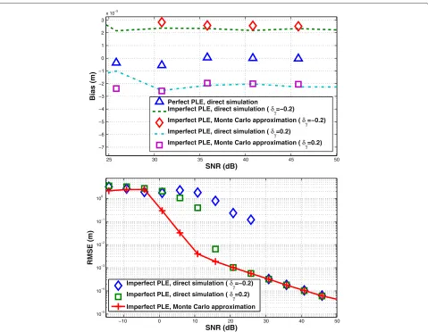
The errors (bias and RMSE) are shown in terms of the transmitter-receiver distanced = cτ for a better display. Figure 6 shows the bias and the RMSE of the estimated distance as a function of received SNR, assuming LOS between the transmitter and the receiver of the commu-nication system. The upper plot shows that the numerical approximation of the bias properly captures the results of the direct simulation for high SNR values and for both positive and negative deviations of the nominal PLE (notice that the range of the vertical axis is only 10−4m). The lower plot shows the Monte Carlo method approxi-mation of the RMSE for a range of SNR values. This figure also shows that a negative deviation of the PLE leads to a greater RMSE than a positive error. This means that the ML estimator of the ToA for a negative PLE mismatch (δγ =γ −γ0<0) is more sensitive to the effects of noise
and shadow fading.
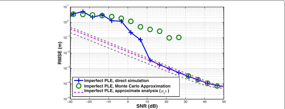
In Figure 7, we show the RMSE of the estimated dis-tance as a function of the received SNR, assuming NLOS between the transmitter and the receiver (hence, with larger values of γ0 andσdB2) and δγ = γ − γ0 = 0.2.
This figure shows that the analytical characterization of the random MSE provided in Section 4.1 is accurate only in the high SNR region. This figure also shows that the Monte Carlo approximation of the RMSE is accurate in the low and the high SNR regions. In the medium SNR region, we observe a larger mismatch.
5.3 Impact of the approximations
In Sections 3 and 4, we have introduced additional approx-imations, beyond the linearization by Taylor series expan-sion, in order to attain analytical expressions for the bias and the MSE of the estimator τˆML(γ ). The goal of this
section is to summarize and point out the impact of such approximations.
In Section 3, we have taken the expectation w.r.t. the noise process n(t) in the denominator of Equation (22). One consequence of this approximation is that the for-mulas in (30) and (37) (for the bias), and (33) and (38) (for the MSE) do not properly capture the effect of the denominator in Equation (22), which is relevant for the performance of the ML estimatorτˆML(γ )in the low SNR region. Although the impact of this approximation cannot be analyzed theoretically, the numerical results in Figure 4 show that the mismatch between the proposed analytical approximation of the RMSE and the RMSE obtained by direct simulation of the communication system is larger in the low SNR region. This artifact is considerably mit-igated when the RMSE is approximated with the Monte Carlo method of Section 4.2. Indeed, it can be seen in Figures 4, 6, and 7 (the latter for a shadow fading sce-nario) that the Monte Carlo estimates of the RMSE are usable in the whole SNR range (although still better for high values, SNR > 20 dB). Note that the Monte Carlo procedure of Section 4.2 requires to draw only from a few simple Gaussian distributions, which is computationally much cheaper than simulating the complete transmission system.
The Taylor series expansion leads to an approximation of the MSE that depends on the sign of the difference δγ = γ − γ0 between the true and the nominal values
of the PLE, as shown in Equation(31). We have followed [23, equation (17-9.6), p. 642] in order to remove this dependence, leading to Equation (32). As a consequence, the analytical and the Monte Carlo approximations of the RMSE proposed in the paper are independent of the sign ofδγ. While this approximation is correct for small δγ, the simulations (see Figures 2, 3, 5, and 6) show
25 30 35 40 45 50 −7
−6 −5 −4 −3 −2 −1 0 1 2 3
x 10−5
SNR (dB)
Bias (m)
Perfect PLE, direct simulation
Imperfect PLE, direct simulation (δγ=−0.2)
Imperfect PLE, Monte Carlo approximation (δγ=−0.2) Imperfect PLE, direct simulation (δγ=0.2)
Imperfect PLE, Monte Carlo approximation (δγ=0.2)
−10 0 10 20 30 40 50
10−5 10−4 10−3
10−2 10−1 100
SNR (dB)
RMSE (m)
Imperfect PLE, direct simulation (δγ=−0.2) Imperfect PLE, direct simulation (δγ=0.2) Imperfect PLE, Monte Carlo approximation
Figure 6Bias (top) and RMSE (bottom) of the estimated distance as a function of the SNR.LOS transmission withγ0=1.7,δγ= ±0.2, σdB2 =1.6,cτ0=4 m,β¯=3.1007×10⁹Hz, sampling time = 0.01 ps, andNR=6, 000 independent runs. Note that the Monte Carlo approximation
of the RMSE is independent of the sign ofδγ.
6 Conclusions
We have analyzed the performance of the maximum like-lihood of a signal time-of-arrival when the path loss expo-nent of the communication link is not perfectly known. In the first approach, we have modeled the signal received amplitude as a deterministic function of the PLE and the transmitter-to-receiver distance. Within this setup, we have applied a Taylor series expansion, together with other approximations needed for mathematical tractabil-ity, in order to obtain closed-form expressions for the bias and the RMSE of the ML ToA estimator. In the second stage, we have extended our analysis to cope with shadow fading effects. In such case, the analyti-cal approximation of the estimator MSE takes the form of a random variable, the mean, variance, and probabil-ity densprobabil-ity function of which are derived and given in closed form. Additionally, we have introduced a simple
Monte Carlo method for the numerical computation of the errors, which removes some of the approximations in the analysis, can be applied both with and with-out shadow fading, and presents a computational load much smaller than that of the direct simulation of the transmission.
−30 −20 −10 0 10 20 30 40 50 10−5
10−4 10−3 10−2 10−1 100 101
SNR (dB)
RMSE (m)
Imperfect PLE, direct simulation
Imperfect PLE, Monte Carlo Approximation Imperfect PLE, approximate analysis ( με2)
Figure 7RMSE of the ML distance estimate as a function of the SNR.NLOS transmission withγ0=3.5,δγ =0.2,σdB2 =7.29,cτ0=4 m,
¯
β=3.1007×10⁹Hz, sampling time = 0.01 ps, andNR=6,000 independent runs. Recall that we have modeled the MSE as a random variable with
meanμε2(Equation (50)) and varianceσ2
ε2(Equation (51)). The analytical approximation of the RMSE of the ML ToA estimation is√με2, and we also
show√με2±σε2in the plot.
in the lower SNR region. The computer experiments also show that the ML ToA estimator is more sensitive to the underestimation of the PLE than to its overestima-tion (this result is consistent with the numerical study of [6]).
Endnotes
a Actually, the negative of the log-likelihood.
b We have solved the optimization problem of
Equation (12) numerically in order to computeτˆML(γ ). In particular, we have generated a regular grid of candidate values ofτ (with separation of 10−2ps between adjacent points of the grid), evaluated the likelihoodfMLfor every candidate, and then selected the
best one. It is not the goal of this paper to propose a practical means for the calculation ofτˆML(γ ), but simply to assess its theoretical performance. In a practical receiver, an adaptive algorithm (similar to a timing error detector [40]) could be used to computeτˆML(γ ).
Appendices
Algebraic derivations
Appendix 1: derivatives of the likelihood functionfML(τ,γ )
The objective of this appendix is to obtain closed expressions for the derivatives of the likelihood function fML(τ,γ ), which are needed in Section 3.2. The partial
derivatives of the likelihood functionfML(τ,γ )w.r.t.τ,τ2,
andγ are given by
∂
∂τfML(τ,γ )= − 1
τγ (Esa−ρ(τ ))a−2a ∂ ∂τρ(τ ),
(66)
∂2
∂τ2fML(τ,γ )= 1
τ2γ (1+γ )Esa 2− 1
τ2γ
1+1 2γ
×aρ(τ)+1 τ2γa
∂
∂τρ(τ)−2a ∂2 ∂τ2ρ(τ),
(67)
∂2
∂γ ∂τfML(τ,γ )= 1
τa(ρ(τ )−Esa)+ 1 τγln
d0
cτ
×a
1
2ρ(τ )−Esa
−ln
d0
cτ
×a ∂
∂τρ(τ ), (68)
respectively, where the correlationρ(τ )can be written as
ρ(τ )= To
0
(r(t)s∗(t−τ ))dt=a0ρss(τ )+ρns(τ ).
(69)
The functionsρss(τ )andρns(τ ), given by Equations (17)
and (18), evaluated atτ =τ0yield
ρss(τ0)= T0
0 |
s(t)|2dt=Es, and (70a)
ρns(τ0)=ρns,0. (70b)
Hence, the expression ofρ(τ )forτ =τ0is given by
Moreover, the derivative of ∂τ∂ ρ(τ ) evaluated atτ = τ0
can be written as
∂
Substituting (71) and (76) into (66) and (68), we obtain the first and the second derivatives, ∂τ∂ fML(τ,γ ) and
The second derivative of the correlation between the transmitted and received signals in (69) w.r.t.τ, forτ =τ0
where the second term is given by
∂2
and the first term can be elaborated as
∂2
in which the first term vanishes, and the change of variable t=t+τ0in the second term yields
The expression of the effective bandwidth in the time
domain is given by β¯ = 2π1
including in (83) the expression of the effective band-width, we have
∂2
can be written as
Finally, substituting (71), (76), and (85) into (67) forτ =
In order to get the expectation w.r.t. the noise of (86), we need the expectations w.r.t. the noise of the correla-tion funccorrela-tion ρns,0 and its derivatives. Fortunately, it is
straightforward to show that
En(t)
Thereby, the expected value of (86) w.r.t. the noise forτ = τ0is given by
Finally, substituting (77), (78), and (88) into (23), we obtain the final expression of the error given in Equation (27).
Appendix 2: derivation of the MSEEn(t)
(εTE(τ0,γ ))2
In this appendix, we derive explicitly a closed formula for the MSE of the ToA estimation based on the Taylor series expansion, i.e., we obtain a closed expression of the MSE in Equation (32). Substituting Equations (24), (25), and (26) into (32) yields
En(t)
By using (87a) and (87b), it is easily shown that the numerator in (89) reduces to
En(t) k1−k2ρns,0+k3ρ˙ns,0
Then, substituting (93a), (93b), and (93c) into (92), we have
and, therefore, plugging (94) into (89), we obtain
En(t)
Finally, substituting the expression of k1,k2, andk3 into
(95), we obtain the final expression of the MSE, given in Equation (33).
Appendix 3: derivation of the effective bandwidth of the second derivative Gaussian pulse
In this appendix, we obtain the effective bandwidthβ¯of the second derivative Gaussian pulse in Equation (64), necessary for the numerical results in Section 4.
where S(ω)is the Fourier transform of the transmitted signals(t). Consider the Fourier transform of the second-derivative monocycle with finite duration pulse from
S(ω)=F{s(t)} = the Fourier transform of the continuous time signals(t).
Assuming that e−2π
S(ω)into two terms, namely
S(ω)=F
Using the time scaling and the frequency properties of the Fourier transform in (98), we obtain
S(ω)=√τp
In order to obtain the effective bandwidth of the trans-mitted signal defined by (96), we need to obtain the value of|S(ω)|2, which is given by
may be rewritten as a function of y in the following equivalent form:
the integral in (103) can be written as
∞
Thereby, by selectingη = τ 2 p
4π andn= 4 and using (104),
the solution of (102) is given by
∞ We start with a straightforward manipulation to obtain
∞
arrive at the solution
∞
Substituting (105) and (107) into (96) yields
¯ therefore, the expression in (108) finally reduces to
¯
Appendix 4: derivation of the effective absolute central frequency of the second derivative Gaussian pulse
Since we work with a carrierless system, we need to elaborate the effective central frequency,
¯
However, it is readily to see that the denominator of (110) is positive (see Equation (105)) while, for the numerator, we obtain
where we have used Equation (104). Therefore, f¯ = 0 and we need to approximate the central frequency by the effective absolute central frequency defined as
¯
Then, we have to evaluate
∞
It is straightforward to show that
∞
and applying the result of (104) into (114), withη = τ 2
Finally, substituting (105) and (115) into (112), we arrive at
¯ signal;n(t), additive noise (zero-mean white Gaussian process with variance σ2
n);Es, energy of the transmitted signal;a=a(τ,γ ), path gain in the model of Section 3.2, which is a deterministic function of the ToA (τ) and the PLE (γ); ψdB, shadow fading variable (assumed Gaussian distributed with zero mean and varianceσdB2);a(ψ ), path gain in the model of Section 4, which is a
random variable that depends on the shadow fadingψ=10ψ10dB and,
deterministically, on the ToA (τ) and the PLE (γ);−fML(τ,γ ), log-likelihood function;ρ(τ ), correlation between the received and the transmitted signals (random variable);ρss(τ ), autocorrelation of the transmitted signal (random variable);ρns(τ ), correlation between the noise and the transmitted signal (random variable);τˆMLandγˆML, ToA and PLE estimates that jointly maximize log-likelihood function−fML(τ,γ );τˆML(γ ), the conditional ML estimator of the ToA obtained for a fixed (but imperfect or mismatched) value of the PLE (γ);εF(τˆML,γˆML), Friedlander’s error in error given in (19);ε˜TE(τ0,γ ), ToA estimation error given in (22), Section 3.2;εTE(τ0,γ ), ToA estimation error given in (23), Section 3.2;B(τ0,γ ), theoretical approximation of the bias of the ToA estimation given in (37), Section 4.1;ε2(τ0,γ,ψ ), theoretical
approximation of the MSE of the ToA estimation given in (41) in Section 4.1, which is a random variable that depends on the shadow fadingψ; ¯
εTE(τ0,γ,ψ ), ToA estimation error given in (53), Section 4.2;ε¯(TEi)(τ0,γ ), sample of the ToA estimation error given in 61, Section 4.2;μN(τ
0,γ ), Monte-Carlo approximation of the bias of the ToA estimation given in (62), Section 4.2; ε2,N(τ
0,γ ), Monte-Carlo approximation of the MSE of the ToA estimation given in (63), Section 4.2;S
N, the signal-to-noise ratio (SNR).
Competing interests
The authors declare that they have no competing interests.
Acknowledgements
Isabel Valera is supported by thePlan Regional-Programas I+DofComunidad de Madrid(AGES-CM S2010/BMD-2422). Bamrung T. Sieskul is grateful to Dr. Feng Zheng and Prof. Dr.-Ing. Thomas Kaiser for partial technical ideas and EUWB research project for financial support during the research period at the Institute of Communications Technology, Leibniz University Hannover, and to Prof. Roberto López-Valcarce for financial support during the research period at the Department of Signal Theory and Communications, University of Vigo. The authors also acknowledge the support ofMinisterio de Economía y Competitividad of Spain (project DEIPRO TEC2009-14504-C02-00 and program Consolider-Ingenio 2010 CSD2008-00010 COMONSENS).
Author details
1Department of Signal Theory and Communications, University Carlos III of Madrid, Madrid, Spain.2Signal Theory and Communications Department, University of Vigo, Vigo, Spain.
Received: 16 November 2012 Accepted: 24 May 2013 Published: 11 June 2013
References
1. S Ping,Delay Measurement Time Synchronization for Wireless Sensor Networks. (Intel Research Berkeley, Berkeley, 2003)
2. Abdulla H, A comparative study of time-delay estimation techniques using microphone arrays. Report No. 619, Department of Electrical and Computer Engineering, The University of Auckland, New Zealand, 2005, pp 1–57
3. G Balogh, Lédeczi Á, M Maróti. Time of arrival data fusion for source localization (Budapest Hungary, 10–14 July 2005)
4. S Gezici, Z Tian, G Giannakis, H Kobayashi, A Molisch, H Poor, Z Sahinoglu, Localization via ultra-wideband radios: a look at positioning aspects for future sensor networks. IEEE Signal Process. Mag.22(4), 70–84 (2005) 5. Y Qi, H Kobayashi, H Suda, On time-of-arrival positioning in a multipath
environment. IEEE Trans. Veh. Technol.55(5), 1516–1526 (2006) 6. V Vivekan, VWS Wong, S Member, Concentric anchor beacon localization
7. J Shirahama, T Ohtsuki, inProceedings of the IEEE vehicular technology conference. RSS-based localization in environments with different path loss exponent for each link (Marina Bay Singapore, 11–14 May 2008) 8. B Sieskul, F Zheng, T Kaiser, A hybrid SS-ToA wireless NLoS geolocation
based on path attenuation: ToA estimation and CRB for mobile position estimation. IEEE Trans. Veh. Technol.58(9), 4930–4942 (2009)
9. Y Chen, E Gunawan, KS Low, SC Wang, CB Soh, LL Thi, Time of arrival data fusion method for two-dimensional ultrawideband breast cancer detection. IEEE Trans. Antennas Propagat.55(10), 2852–2865 (2007) 10. BT Sieskul, F Zheng, T Kaiser, inProceedings of the 10th IEEE international
workshop on signal processing advances in wireless communications 2009 (SPAWC 2009). Time-of-arrival estimation in path attenuation (Perugia, Italy, 2009)
11. G Mao, BD Anderson, B Fidan, Path loss exponent estimation for wireless sensor network localization. Comput. Netw.51(10), 2467–2483 (2007) 12. ZZ Ruisi He, J Ding, An empirical path loss model and fading analysis for
high-speed railway viaduct scenarios. IEEE Antennas Wireless Propagat. Lett.10, 808–812 (2011)
13. X Zhao, L Razoumov, LJ Greenstein, Path loss estimation algorithms and results for RF sensor networks. Proc. IEEE Veh. Tech. Conf.7, 4593–4596 (2004)
14. S Srinivasa, M Haenggi, inProceedings of the IEEE information theory and applications workshop (ITA ’09). Path loss exponent estimation in large wireless networks (San Diego, CA, 2009)
15. T Mogi, T Ohtsuki, in14th Asia-Pacific conference on communications (APCC). ToA localization using, RSS weight with path loss exponents estimation in NLOS environments (Tokyo, Japan, 2008)
16. N Benvenuto, F Santucci, A least squares path-loss estimation approach to handover algorithms. IEEE Trans. Veh. Technol.48(2), 437–447 (1999) 17. CD Richmond, inProceedings of the fourth IEEE workshop on sensor array
and multichannel processing (SAM). On the threshold region mean-squared error performance of maximum-likelihood direction-of arrival estimation in the presence of signal model mismatch (Waltham, MA, 2006) 18. B Friedlander, Sensitivity analysis of the maximum likelihood
direction-finding algorithm. IEEE Trans. Aerosp. Electron. Syst.26(6), 953–968 (1990)
19. A Goldsmith,Wireless Communications. (Cambridge University Press, London, UK, 2005)
20. Y Qi, H Kobayashi, H Suda, Analysis of wireless geolocation in a non-line-of-sight environment. IEEE Trans. Wireless Commun.5(3), 672–681 (2006)
21. D Slepian, Estimation of signal parameters in the presences of noise. IRE Trans. Inform. Theory.3, 68–89 (1954)
22. P Swerling, Parameter estimation for waveforms in additive Gaussian noise. J. Soc. Indust. Appl. Math.7(2), 152–166 (1959)
23. H Urkowitz,Signal Theory and Random Processes. (Artech House, Washington, MA, 1983)
24. HV Poor,An Introduction to, Signal Detection and Estimation, 2nd edn. (Springer, New York, 1994)
25. CW Helstrom,Elements of, Signal Detection and Estimation. (Prentice Hall, Englewood Cliffs, NJ, 1995)
26. RN McDonough, AD Whalen,Detection of, Signals in Noise, 2nd edn. (Academic, New York, 1995)
27. HL Van Trees,Detection, Estimation, and Modulation, Theory, Part I Detection, Estimation, and Linear Modulation Theory. (Wiley, New York, 2001) 28. RD Hippenstiel,Detection theory: Applications and Digital Signal Processing.
(CRC Press, Boca Raton, Florida, 2002)
29. BC Levy,Principles of, Signal Detection and Parameter Estimation. (Springer, New York, 2008)
30. TS Rappaport,Wireless Communications: Principles and, Practice, 2nd edn. (Prentice-Hall, Englewood Cliffs, 2002)
31. K Sharman, T Durrani, M Wax, T Kailath, inProceedings of the IEEE conference on acoustics, speech, and signal processing (ICASSP). Asymptotic performance of eigenstructure spectral analysis methods (San Diego, CA, 1984)
32. P Stoica, A Nehorai, MUSIC, maximum likelihood and Cramér-Rao bound. IEEE Trans. Acoust., Speech, Signal Process.37(5), 720–741 (1989) 33. M Viberg, B Ottersten, Sensor array processing based on subspace fitting.
IEEE Trans. Signal Process.39(5), 1110–1121 (1991)
34. JAC Brown, J Aitchison,The Lognormal Distribution. (Cambridge University Press, UK, 1963)
35. BT Sieskul,NLoS Localization and UWB Channel Capacity Analysis (Hannoversche Beiträge zur Nachrichtentechnik / 2:
Kommunikationsnetze) (Shaker, Germany, 2010)
36. CP Robert, G Casella,Monte Carlo statistical methods. (Springer, New York, 2004)
37. Z Sahinoglu, S Gezici, I Guvenc,Ultra-Wideband Positioning, Systems Theoretical Limits, Ranging Algorithms, and Protocols. (Cambridge University Press, UK, 2008)
38. S Ghassemzadeh, R Jana, C Rice, W Turin, V Tarokh, Measurement and modeling of an ultra-wide bandwidth indoor channel. Commun. IEEE Trans.52(10), 1786–1796 (2004)
39. MZ Win, RA Scholtz, Ultra-wide bandwidth time-hopping spread-spectrum impulse radio for wireless multiple access communications. IEEE Trans. Commun.48(4), 679–691 (2000)
40. U Mengali,Synchronization Techniques for Digital Receivers. (Springer, New York, 1997)
doi:10.1186/1687-1499-2013-158
Cite this article as:Valeraet al.:On the maximum likelihood estimation of the ToA under an imperfect path loss exponent.EURASIP Journal on Wireless
Communications and Networking20132013:158.
Submit your manuscript to a
journal and benefi t from:
7 Convenient online submission 7 Rigorous peer review
7 Immediate publication on acceptance 7 Open access: articles freely available online 7 High visibility within the fi eld
7 Retaining the copyright to your article