R E S E A R C H
Open Access
Two-hop time synchronization protocol for
sensor networks
Jing Wang
*, Shuai Zhang, Dan Gao and Yingguan Wang
Abstract
One of the critical middleware services for sensor networks is the time synchronization, which provides supports to different applications. Synchronization protocols used for Internet and LANs are not appropriate in the sensor networks for the high-density and limited energy resource. This paper describes two-hop time synchronization (TTS) that aims at reducing the synchronization overhead and providing more accurate network-wide synchronization. The synchronization message exchanges are minimized by making full use of sensors’ broadcast domain and enlarging the common node synchronization range in multi-hop scenarios. By halving synchronization hops, the TTS achieves high multi-hop synchronization precision. The proposed protocol contains single-hop synchronization model, multi-hop synchronization algorithm, and a power control scheme. We prove that the extension of single-hop TTS to network-wide synchronization is NP-complete. The complexity and convergence time of multi-hop TTS are analyzed in detail. We simulate TTS on MATLAB and show that it requires minimal overhead and convergence time compared with other protocols. We also implement TTS on common sensors and its multi-hop synchronization error is less than that of receiver-receiver synchronization (R-RS).
Keywords: Sensor networks; Time synchronization; Synchronization hops; Synchronization range; Multi-hop
1 Introduction
The technological advances in miniaturization, in digi-tal circuits design, and in wireless communication are promoting the study of sensor networks with small and low-cost nodes. By interacting with the environment and communicating with each other, the sensors could provide future ubiquitous communications. When those sensor nodes are deployed over a wide geographical region, they form the wireless sensor networks (WSN). They are use-ful for providing applications varying from environment monitoring to equipment monitoring, from smart office to industrial automation [1].
Clock synchronization is one of the most important components in WSN. It is essential for transmission scheduling, power management, data fusion, and many other applications. For example, in power management, the duty cycling helps the sensors to maintain energy by consuming minimal power during the sleep mode. The performance of duty cycling is closely related to the accuracy of the whole network synchronization.
*Correspondence: [email protected]
Shanghai Institute of Microsystem And Information Technology, Chinese Academy of Sciences, Shanghai 201899, China
Although the time synchronization problem has been solved in common networks, it requires to be reconsid-ered in WSN. First, such networks are energy constraint, so the time synchronization protocol must be energy effi-cient. Second, nodes in sensor networks communicate with each other via multi-hop paths. The single-hop error accumulates along the synchronization hops, and the multi-hop error is inevitable. Sometimes, the multi-hop synchronization error even becomes a major considera-tion due to the large network scale.
1.1 Our contribution
We propose the single-hop TTS to solve the disadvan-tages of traditional synchronization models. The model has the same time accuracy with receiver-receiver syn-chronization (R-RS), and its reference node can also be synchronized. Our main contribution is the multi-hop TTS protocol, which is the extension of single-hop TTS. We prove that this extension process is NP-complete and present a new distributed algorithm to accomplish it. The fundamental property of multi-hop TTS is that it synchro-nizes nodes within two adjacent levels in one synchroniza-tion process. In our design, reference node and its parent
node perform two-way timing message exchange to syn-chronize nodes lying within the reference node broadcast domain. The TTS minimizes the reference nodes needed to cover the entire network and has the largest com-mon node synchronization range in multi-hop scenarios. So it could reduce multi-hop synchronization overhead significantly. Our approach decreases multi-hop synchro-nization error by halving the synchrosynchro-nization hops. We analyze the complexity and convergence time of multi-hop TTS, and the result shows that our work is simple and fast. Odd layer TTS, which uses odd layer nodes as the reference nodes, is another achievement of this paper. This scheme is used to balance the energy consumption of nodes in different levels.
2 Related work and challenges
The most important single-hop synchronization mod-els are receiver-receiver synchronization, pair-wise syn-chronization (P-WS) and sender-receiver synsyn-chronization (S-RS).
In R-RS, different nodes that receive the same ref-erence message can be synchronized with each other by exchanging the recorded reception time. References [2,3] and [4] are based on reference broadcast synchro-nization (RBS) which is the most important prototype of R-RS. RBS achieves higher time accuracy compared with other protocols by removing the non-determinism of the sending end. However, in RBS, the reference node is left unsynchronized.
P-WS uses pair-wise message exchanges to achieve the synchronization of two adjacent nodes. Protocols that adopt this model are lightweight time synchronization (LTS) [5], tiny-sync and mini-sync [6], and timing-sync protocol for sensor networks (TPSN) [7].
S-RS synchronizes a receiver with a sender by broad-casting multiple time packets. The flooding time synchro-nization protocol (FTSP) [8] and delay measurement time synchronization (DMTS) [9] analyze the sources of uncer-tain delay in message exchange in detail. FTSP utilizes media access control (MAC) time stamping to minimize the clock offset. It also adopts linear regression to com-pensate the clock skew.
Recently, some new protocols have been proposed to solve the drawbacks of the above models. In pair-wise broadcast synchronization (PBS) [10], a node gets syn-chronized by overhearing the exchanged messages from two neighbors. In vector Kalman filter using multiple parents (KFMP) [11], a node combines the messages from multiple parents and adopts vector Kalman filter to reduce the global clock error. The master synchronization [12] adopts physical layer feedback control to save power consumption. Recently, a new approach called Average TimeSynch (ATS) [13] is proposed to estimate the clock
offset and skew by utilizing distributed low-pass filter. Although some multi-hop protocols have been proposed to fit the above models, the multi-hop clock synchro-nization is still challenging for several reasons. On one hand, the synchronization hops become a major consider-ation for better clock protocols design. This is because the multi-hop synchronization error accumulates along the hops. For example, RBS proves that the multi-hop error increases with the square root of the hops. In order to reduce the cumulative multi-hop error, most algorithms focus on designing more accurate single-hop model or adopting a statistical signal processing framework. How-ever, we find that all the current multi-hop protocols virtually share the same synchronization hop: the least hop to the root node. So our work aims at reducing the synchronization hops and providing precise multi-hop synchronization.
Synchronization overhead is another challenge that multi-hop synchronization faces due to the limited power sources. Actually, the overhead (energy consumption) is the opposite of time accuracy. The three basic mod-els focus on improving the synchronization accuracy, so their synchronization overheads are usually very large. In [14] and [15], some multi-hop extensions of PBS have been devised. The extensions aim to minimize the num-ber of synchronization packets. However, their effects are unsatisfactory because the synchronization range of PBS is too small. Synchronization range is the key factor for the energy-efficient protocol design. No protocol notices that, in multi-hop synchronization, the synchronization range of a common node is smaller than the single-hop synchronization range.
3 The single-hop model of TTS
The TTS is designed to achieve the synchronization of the whole network. In general, the communication radius of a sensor is assumed to be less than a few hundred meters. In this case, the propagation delay can be ignored. Since the energy consumption increases with the broad-cast radius, this assumption is consistent with common sensor networks.
The single-hop TTS focuses on providing synchroniza-tion points (sync-points), which can be used to estimate the node clock phase and skew, instead of the approach to calculate the offsets directly.
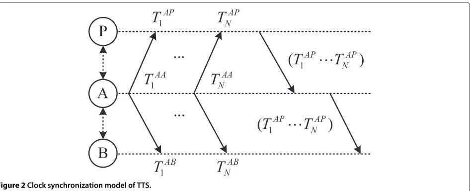
In Figure 1a, suppose thatPis a parent node andAis a reference node. Common nodeB, which lies within the broadcast region ofA, collects sync-points by overhearing the information fromA. The message exchange model is depicted in Figure 2.
+
(a)
(b)
Figure 1Synchronization examples of TTS and traditional protocols.(a)Synchronization example of TTS.(b)Synchronization example of traditional protocols.
2. Each receiver records the time stamp at reference message reception. The reception time ofP and B areTiAPandTiAB, respectively.
3. P forwards a packet containing N recorded time stamps toA.
4. A broadcasts the packet received from P.
From Figure 2,T1APandTiAPcan be expressed as
T1AP=T1AB+θoffsetBP +c+1 (1)
TiAP=TiAB+θoffsetBP +θskewBP ·(TiAB−T1AB) +c+i, 1<i≤N
(2)
whereθoffsetBP andθskewBP denote the clock offset and skew betweenBandP. The parameterscandi stand for the
fixed portion and random portion of packet delay [2,7,8]. If the set of time stamp differences is denoted byT =
T1AP−T1AB· · ·TNAP−TNABT, then it can be expressed as follows:
T =H+C+E (3)
where=θoffsetBP θskewBP T,C=[c· · ·c]T,E=[1· · ·N]T,
andH=
1 1 · · · 1
0 T2AB−T1AB · · · TNAB−T1AB T
.
Consequently, using the Equation 3,Bcan be synchro-nized withP. In addition, Equations 1 to 3 can also be used to synchronize the reference node by substitutingA forB. In order to improve the precision, TTS usesN+2 broadcast packets to provideNsync-points and the node records time stamp at MAC layer to remove send, receive, and access time. It is worth mentioning thatButilizes ref-erence broadcast scheme to eliminate the transmitter-side non-determinism, thusBPi ≈iAP/2.
4 The multi-hop algorithm of TTS
In practical WSN, a common node always gets informa-tion from the root node through a multi-hop path. Thus, the single-hop TTS is not enough to achieve the whole network synchronization. In these scenarios, the multi-hop TTS should be used to synchronize nodes beyond the communication range of the root node.
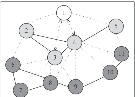
We utilize a simple demo illustration to show the differ-ence between common protocol and multi-hop TTS. In Figure 3, suppose that only root node 1 has the global time. For common protocols, first, the root node synchronizes the four nodes connected with it. Then, nodes 3 and 4 are selected to synchronize nodes of level 3. However, TTS only selects two pairs of nodes to synchronize all com-mon nodes. For example, nodes 3 and 1 perform pair-wise message exchange to synchronize nodes 2, 3, 4, 6, 7, 8, and 9 because they all locate within the broadcast range of node 3. Similarly, nodes 4 and 1 exchange packets to syn-chronize nodes 2, 3, 4, 5, 8, 9, 10, and 11. Therefore, the TTS aims at finding all the synchronization pairs from the whole network.
Figure 3Network-wide TTS synchronization for a simple network.
4.1 Synchronization problem formulation
The procedure of searching synchronization pairs can be divided into some sub-problems. Suppose that reference nodes of level 2i−2 have been found whereas reference nodes of level 2iare not found. This means that nodes of level 2iand 2i+1 are uncovered. We utilize an undirected graphG(V,E)to model the topology of nodes of level 2i and 2i+1. LetV =VE∪VOrepresent the set of nodes.VE
is the set of level 2inodes andVO is the set of level 2i+
1 nodes. Edge setEstands for the set of communication link and node self-loop. The link(v,e) ∈ Eif it satisfies: at least one of the two elements belongs toVE, vcould
communicate witheorv=e. Thus, the edges connecting nodes inVOonly are not included. Then, the sub-problem
can be described as finding minimum number of reference nodes fromVEto cover all nodes inV.
Theorem 1. The process of the sub-problem is
NP-complete.
Claim 1.The sub-problem is in NP.
Proof. The following verifier for the sub-problem runs in polynomial time.
For(V,E,K),R
If all the followings are all true then accept else reject: Ris a subset ofVE
|R| ≤K
∀v∈V∃e∈R[(v,e)∈E].
Claim 2.Set covering problem (SCP)≤ psub-problem
Proof. Suppose a function with the input (V,S,K), which is a SCP instance, and output (V,E,K) which
stands for the sub-problem. Let S = {Se : e ∈ VE}
andSe = {v ∈ V : (v,e) ∈ E}. There are |V|vertices
and|eS=|1|Se|edges. We now show that the function is a
polynomial time reduction of SCP to sub-problem. We assume thatJis a S-cover ofVand letR= {e∈VE :
Se ⊂ J}. Suppose|J| = K, then|R| = K. We claim that
Rcould cover all elements ofV. Supposevis a common node ofV. So we have{v∈Se:Se⊂ J}. According to the
definition ofSe,(v,e)∈ E. The definition ofRshows that
e∈R. Thus,vcould be covered by an elementeofR. Then, we supposeRwith size ofK could cover all the elements ofV. letJ = {Se :e∈ R}, then|J| =K. We will
show thatJis a S-cover ofV. For a common nodev∈V, we know that∃e ∈ R[(v,e)∈E]. Thus, according to the definition ofSe,v∈Se. The definition ofJshows thatSe∈
J. We can see thatv∈JandJis the cover ofV.
4.2 Multi-hop process of TTS
There is no efficient way to solve the SCP. A famous sub-optimal solution for SCP is the greedy algorithm. We propose the multi-hop TTS, which is a distributed greedy algorithm, to solve the sub-problem. This algorithm only uses even layer node as reference node, so it is also named as even layer TTS.
Every node in the network is assigned a unique ID to identify the source of message. A node obtains its level through the level discovery phase [7]. The parameter synv represents the cover state of nodev, that is, synv=1 when v itself is the reference node or vis located within the broadcast domain of a reference node, and synv= 0 oth-erwise. Let numvdenote the number ofv’s neighbors with
parameter syn=0. The variable num can also be obtained initially from the level discovery phase. The distributed algorithm can be described as:
1. Nodes inVEare divided into two types, reference
nodes and common nodes. According to CSMA, common nodee∈VEwaits for some random time to
avoid collision and to ensure that the wireless channel is free. Then,e broadcasts a packet containing numeand its own identity. Meanwhile,e
also collects corresponding variables from the neighbors. Having received all such variables,e computes out and broadcasts the maximum value {maxe=max(numv),v∈VE,(v,e)∈E}to all the
neighbors. In this step, the number of broadcasted messages is less than2|VE|.
2. Common nodee∈VEjudges whether it needs to be
a reference node or remains a common node. Nodee becomes a candidate of the reference node if numeis
the largest variable among all the two-hop neighbors ofe. That is,
If candidatee timeouts after some random time without receiving any reference message (refmsg), it becomes a reference node and broadcastsrefmsg immediately. Otherwise, nodee is still a common node.
Here, we present a simple example of this step. In Figure 3, suppose that all nodes of levels 2 and 3 are uncovered, that is, their parameters syn are all equal to zero. Now the sub-problem is to find all the reference nodes of level 2. First, every node of level 2 exchanges num with the neighbors of the same level. From Figure 3, we can see that num2=| {2, 3, 4, 6} |= 4, num3=| {2, 3, 4, 6, 7, 8, 9} |=7, num4=| {2, 3, 4, 5, 8, 9, 10, 11} |=8, num5=| {4, 5, 11} |=3. Then, node 4 becomes a reference node because num4is the largest among all the neighbors. The iterative process continues until nodes 6 and 7 are also covered.
3. If nodev∈Vwith parameter synv=0becomes a reference node or has receivedrefmsg, it sets the parameter synv=1and broadcasts a cover state message (covstate). This broadcasting process also adopts CSMA scheme.
Steps 1 to 4 are repeated until all nodes in V are lying within the broadcast range of the reference nodes. Then, each reference node randomly selects a level 2i− 1 neighbor to make a synchronization pair, and this sub-problem is finished. When all these sub-problems have been accomplished, the network-wide synchro-nization will be performed along the synchrosynchro-nization pairs.
4.3 The performance of multi-hop TTS
Theorem 2. The multi-hop TTS yields a set of size at most ln+2times the size of the optimal set.
Proof.See Appendix.
In multi-hop TTS, more than one reference node is found in one iteration process and only a small num-ber of nodes become reference nodes. Hence, the actual number of iterations is far less than|VE|and the
max-imum complexity of step 1 is O(|VE|2). In steps 2 and
3, every node broadcasts the messagecovstateand some nodes broadcast the message refmsg, so the complexity is O(|V|). Therefore, the total complexity of the whole process is{O(|VE|2)+O(|V|)}. Note that the
communi-cation messages needed to determine the synchronization pairs are one-off.
The TTS reduces the synchronization messages sig-nificantly because it makes full use of node’s broadcast characteristic. A node’s broadcast range can be divided into three parts: area that covers neighbors in the previ-ous layer, area that covers neighbors in the same layer, and area that covers neighbors in the next layer. In common protocols, a synchronized node can only synchronize its neighbors in the next layer. However, the reference node of TTS is able to synchronize all neighbors in the same and next layer. Therefore, the broadcast domain utiliza-tion of TTS is higher than that of common protocols. As depicted in Figure 1a,b, TTS gives a roughly 2× larger maximum synchronization area compared with other pro-tocols. Moreover, the distributed TTS chooses the most appropriate nodes as the reference nodes. By minimiz-ing reference nodes, TTS significantly reduces the number of timing packets which are heavy overheads in terms of energy consumption.
The TTS halves the synchronization hops and effec-tively reduces the multi-hop synchronization error by synchronizing nodes of two adjacent levels. In Figure 1a,b, suppose that bothP andP have been synchronized and the number of hops from a common node to the root node isH. The goal of traditional protocols is to ensure the shortest path, which means the least number of hops, to the root node. They useP of levelito synchronize the nodes of leveli+1. Thus, the number of synchronization hops of traditional protocols isH. However, TTS selectsP of level 2i−1 andAof level 2ias a synchronization pair to synchronize level 2iand 2i+1 nodes. The number of syn-chronization hops of TTS can be expressed as [(H+1)/2], which means the floor of(H+1)/2, i.e., the largest integer less than or equal to(H+1)/2. Since the synchronization error increases with the number of synchronization hops, the accuracy of TTS is higher compared with previously known protocols.
Fewer synchronization hops and less overhead mean lower convergence time that is needed to achieve
network-wide synchronization. Let C be the channel
capacity,ρbe the node density, andrbe the node broad-cast radius. Then, the node throughput equalskC/(πr2ρ) where kis the channel utilization. Traditional protocols exchangeN timing packets to accomplish synchroniza-tion, and reference [2] shows that the most suitable value ofNis 30. The convergence time of traditional protocols can be expressed as:
CTt=
πr2P
kC ρtNHmax (6)
2 4 6 8 2
4 6 8
N(the number of sync messages)
(a)
Hmax(the maximum hops)
2 4
6 8 10
1 3 5 7 9 −10
0 10 20 30 40
N Hmax
The calculated difference
(b)
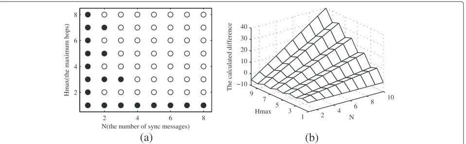
Figure 4The comparison and difference betweenNHmaxand(N+2)[(Hmax+1)/2].(a)The comparison ofNHmaxand(N+2)[(Hmax+1)/2].
The white dot represents that the former is larger than the latter and the black dot conversely.(b)The difference betweenNHmaxand
(N+2)[(Hmax+1)/2].
are half of that of common protocols. The convergence time of TTS is given by:
CTeTTS= πr2P
kC ρeTTS(N+2)[
Hmax+1
2 ] . (7)
Equations 6 and 7 show that the convergence time raises with the increasing of the value ofρ. As shown earlier, TTS requires less synchronization nodes to synchronize the whole network and thus ρeTTS < ρt. So TTS has
less convergence time when just considering about the parameterρ. In addition, the parameterkdecreases with the growth of ρ in basic CSMA which is a very impor-tant MAC layer protocol [16,17]. Then, we assumeρt =
ρeTTSand compareNHmaxwith(N+2)[(Hmax+1)/2]. We turn to MATLAB to verify TTS has less convergence time. In Figure 4a, the white dot denotes that NHmax is relative large. When the number of N is larger than 3, the TTS always has less convergence time compared with common protocols in multi-hop networks. Actually, in order to calculate the clock skew,Nis usually very large. Figure 4b plots the calculated difference betweenNHmax
Figure 5Example of the power control scheme as an application service.
and(N+2)[(Hmax+1)/2]. The figure shows that the dif-ference increases with the growths of both NandHmax. Therefore, TTS performs better in networks with large maximum number of hops.
4.4 Power control scheme
In WSN, nodes have to work as energy-efficient as possi-ble due to limited energy supply. In the protocol proposed above, only even layer nodes are chosen as reference nodes. Those selected nodes consume more power com-pared with odd layer nodes. Here, we present odd layer TTS to solve this problem.
The root node broadcasts N packets containing the sender’s time stamps which denote the global time. Each level 2 node obtains the corresponding local time at message reception. The node calculates the clock offset by working out the difference between the global and local time and then becomes synchronized. Nodes of
3 5 7 9 11 13 15 0
2000 4000 6000 8000 10000
The length of the network (L)
(a)
Number of synchronization messages
Even layer TTS Odd layer TTS FTSP TPSN
3 5 7 9 11 13 15
0 0.2 0.4 0.6 0.8 1
The length of the network (L)
(b)
Normalized convergence time
TTS FTSP TPSN
Figure 7Message overhead and convergence time of different protocols.(a)The message overhead differences between different protocols. (b)The convergence time differences between different protocols.
level 2 are synchronized by S-RS which has lower accu-racy compared with R-RS. After that, odd level nodes use the above distributed algorithm to achieve network-wide synchronization. Note that even layer TTS and odd layer TTS can be performed alternately in practical WSN protocols.
Figure 5 shows a possible way of achieving power con-trol by utilizing two types of TTS. Each synchronization node with less power remaining sends a warning message containing its own identity and level to the root node. An application PowerControl is generated by the root node to collect the energy consumption state of the whole network.PowerControlanalyzes the data and changes the synchronization mode when the powers of most current reference nodes are too low. Then,PowerControl starts a flooding process to notify all the nodes. Depending on the judgment ofPowerControl,SynAPPinitials the whole network synchronization.
5 Experiment results
5.1 Message overhead and convergence time comparison
The experiment scenario is a L∗ L network with grid topology, in which each node communicates with the
Figure 8Close-up of the common sensor node.
neighbors only. An example of the topology connection state is shown in Figure 6. The gray dot deployed in the upper right corner is the root node. The white dot denotes the reference node which connects with its par-ent node via dashed line. The reference node and parpar-ent node makes a synchronization pair, and all synchroniza-tion pairs are selected by even layer TTS. In the figure, only the most appropriate even layer nodes are chosen as reference nodes, and all nodes could be located within the broadcast domain of the synchronization pairs. The next experiment focuses on the overhead and convergence time required by different protocols.
We evaluate the message overhead required by TTS, TPSN, and FTSP. In TPSN, each node except the root node forms a synchronization pair with its parent and each synchronization pair demands 2Ntiming messages. Therefore, TPSN needs 2N(L2−1)packets to achieve syn-chronization of the network mentioned before. If FTSP is adopted to synchronize the network, every node sends its time stamp to other nodes, so the number of required packets is NL2. Notice that RBS demands O(L4) pack-ets in a single-hop network, which is too large compared with both TPSN and FTSP. The value of N is set to be 20. It can be seen from Figure 7a that TTS requires a much lower number of overheads compared with both TPSN and FTSP. The overhead gaps between TTS and other protocols become greater asL is increasing. This indicates that TTS performs better with regard to energy consumption versus TPSN and FTSP in large-scale net-works. Furthermore, the decrease of packets also means the reduction of network conflict and global time error.
Figure 9Wireless sensor network communication topology of ten sensor nodes.
just simulated TPSN, FTSP, and TTS on MATLAB. In the simulation, the TPSN first established a tree hierar-chy and each node synchronized with its parent through pair-wise message exchange. The FTSP achieved network-wide synchronization by flooding. In all the three proto-cols, common nodes communicated with their neighbors through CSMA protocol. Figure 7b shows the conver-gence times of different protocols. Each point represents the average of 100 experiment results. The convergence times of the three protocols all increase with the network size because the number of nodes and maximum hops increase with the network scale. The convergence time of TTS is always less than the other two protocols and
the gaps raise with L. This is consistent with Equations 6 and 7. The reason lies in two aspects: TTS has less message overhead; TTS halves the synchronization hops. Therefore, TTS converges fast and performs significantly better in large-scale WSN.
5.2 The synchronization accuracy of TTS
We use the implementation of TTS on common sensors to carry out the advantages of TTS described above. The hardware of the sensor consists of processor board, radio, and battery. We base our design on the microcontroller TI MSP430F5438 and on the radio chip TI CC1100E. The processor adopts 16 MHz external crystal oscillator, so its timer maintains a local clock with the resolution of about 0.0625 μs. The central frequency of the radio chip is 470 MHz, and its data rate is set to be 100 kBaud. We uti-lize the 4.5-V lithium rechargeable battery as the power of the sensor. The sensor also provides lots of external inter-faces (e.g., RS232 serial port, JTAG emulator interface, LED lights). Figure 8 shows a prototype of this hardware design.
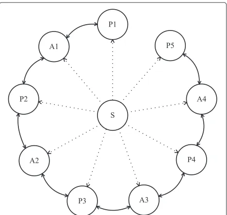
Figure 9 shows the experiment scenario and the net-work connection state. The experiment involves a super node and nine common nodes. The topology of the ten nodes is enforced in software in order to facilitate the realization. The topology structure shows that all com-mon nodes could be covered by the broadcast domain of the super node S. S queries and collects the clock time fromPi once per 7.9 s. It sends the time readings to PC
through 115, 200-baud serial link. Then, S broadcasts a start message, so that all nodes begin to re-synchronize. The synchronization process is started by the root node P1which maintains the global time. Other common nodes communicate with the neighbors and exchange synchro-nization messages according to the adopted protocols demonstrated below.
0 0.2 0.4 0.6 0.8 1 1.2
0.2 0.4 0.6 0.8 1
Synchronization error (µsec)
(a)
Cumulative error probability
Multi−hop synchronization error of TTS
2 hop 4 hop 6 hop 8 hop
0 0.4 0.8 1.2 1.6
0.2 0.4 0.6 0.8 1
Synchronization error (µsec)
(b)
Cumulative error probability
Multi−hop synchronization error of R−RS
2 hop 4 hop 6 hop 8 hop
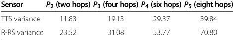
Table 1 Statistics of synchronization variances over multi-hop
Sensor P2(two hops)P3(four hops)P4(six hops)P5(eight hops)
TTS variance 11.83 19.13 29.37 39.84 R-RS variance 23.52 31.08 53.77 70.80
• TTS:PiandAiexchange messages, andPi+1 synchronizes withPiby overhearing the broadcasts
fromAi. After that,Pi+1starts to exchange messages withAi+1. This process continues untilP5is
synchronized.
• R-RS: At first,S broadcasts a reference message.P1 andA1records the reception time; then,P1sends the recorded time toA1.A1synchronizes withP1by computing out the time difference. This process continues untilP5is also synchronized withA4.
Each scenario consists of 500 trials. We compute out the synchronization error between P1 and Pi. The
dis-tributions of clock error are shown in Figure 10, and the variances are summarized in Table 1. As shown in Figure 10a,b, the synchronization error increases with hop distance. This means that, both in TTS and R-RS, nodes with lower hops perform better than those with higher hops. The thresholds at confidence of 90% in two, four, six, and eight hops of TTS are about 0.36, 0.43, 0.52, and 0.60 μs, respectively. The values of TTS are better than that of the R-RS (0.48, 0.59, 0.75, and 0.84 μs). From Table 1, the four-hop variance of TTS is smaller than the two-hop vari-ance of R-RS. Although the eight-hop varivari-ance of TTS is larger than the four-hop variance of R-RS, they are in the same order of magnitude and the former is smaller than the six-hop variance of R-RS. In summary, TTS dramati-cally reduces the variance of global synchronization error. The reason is that TTS halves the synchronization hops.
6 Conclusions
In this paper, we have introduced the two-hop time syn-chronization for sensor networks. We show that TTS requires less message exchanges to achieve network-wide synchronization. The efficacy of this claim is verified via simulations on MATLAB. The convergence time of TTS is also very low. We argue that TTS is more accurate in large-scale networks because it halves synchronization hops. We verify this claim by implementing TTS and R-RS on common sensors. The results show that TTS performs better than R-RS in multi-hop synchronization.
The single-hop TTS can be used as the substitute of R-RS. In TTS, the reference node records the time stamps when broadcasting reference messages. The reference node and its children nodes can be synchronized with a selected parent node. We utilize a distributed algorithm to
extend the single-hop TTS to multi-hop synchronization. The algorithm minimizes the number of reference nodes and halves the synchronization hops compared with other protocols. Thus TTS is a distributed, scalable, energy-efficient, and accurate solution to the problem of sensor network clock synchronization.
Our future work will focus on several aspects. First, TTS is sensitive to the dynamic topology change, so we would like to make it more robust. Then, we plan to verify the performance of TTS in a real-world application. The most attractive scenarios are those with great range of hardware platforms, time-varying network topology, and multi-user applications.
Appendix
Theorem 3. The multi-hop TTS yields a set of size at most ln+2times the size of the optimal set.
Proof.Suppose that OPT ⊂ VE is the optimal set. A
node inVeither belongs to OPT or has a neighbor in OPT. The set of nodes covered byi∗ ∈ OPT is calledSi∗. If a
node is covered by more than one neighbors in OPT, we arbitrary assign it to one of such sets.
We use the charging scheme to prove the efficacy of TTS. The total cost of an optimal setSi∗is 1 and each node
of the set is charged 1/|Si∗|. In the following, we prove that
the total cost of TTS is at most ln+2 for each setSi∗.
Each time we select a reference node, we charge the new nodes that become covered in this step. A node is charged only once because it gets covered only once. Suppose the number of nodes covered by a new reference nodeiisNi.
Then, if node vin the set ofSi∗ is covered by i, it gets
charged 1/Ni. According to step 1 of multi-hop TTS,Ni
is the largest among all the two-hop neighbors and there-fore Ni > Ni∗. So node vgets charged at most 1/Ni∗.
Let di∗ represent the number of neighbors of node i∗.
Therefore, the first node in the set ofSi∗gets charged at
most 1/(di∗+1) and thejth node gets charged at most
Competing interests
The authors declare that they have no competing interests.
Acknowledgements
This work is supported in part by the ‘Strategic Priority Research Program’ of the Chinese Academy of Sciences (CAS) under Grant No. XDA06020301 and Shanghai Science and Technology Commission (SSTC) research projects under Grant No. 12DZ2293200.
Received: 1 July 2013 Accepted: 7 March 2014 Published: 12 March 2014
References
1. F Wang, P Zeng, H Yu, Y Xiao, Random time source protocol in wireless sensor networks and synchronization in industrial environments. Wireless Commun. Mobile Comput.13(8), 798–808 (2013)
2. J Elson, L Girod, D Estrin, Fine-grained network time synchronization using reference broadcasts. SIGOPS Oper. Syst. Rev.36(SI), 147–163 (2002) 3. S PalChaudhuri, AK Saha, DB Johnson, Adaptive clock synchronization in
sensor networks, inProceedings of the 3rd international symposium on
Information processing in sensor networks(ACM IPSN ’04, New York, NY,
USA, 2004), pp. 340–348
4. A Marco, R Casas, J Ramos, V Coarasa, A Asensio, M Obaidat,
Synchronization of multihop wireless sensor networks at the application layer. Wireless Commun. IEEE.18, 82–88 (2011)
5. J van Greunen, J Rabaey, Lightweight time synchronization for sensor networks, inProceedings of the 2nd ACM international conference on
Wireless sensor networks and applications(ACM WSNA ’03, New York, NY,
USA, 2003), pp. 11–19
6. ML Sichitiu, C Veerarittiphan, Simple, accurate time synchronization for wireless sensor networks, inWireless Communications and Networking
Conference, vol. 2 (IEEE WCNC ’03, New York, NY, USA, 2003),
pp. 1266–1273 vol. 2
7. S Ganeriwal, R Kumar, MB Srivastava, Timing-sync protocol for sensor networks, inProceedings of the 1st international conference on Embedded
networked sensor systems(ACM SenSys ’03, New York, NY, USA, 2003),
pp. 138–149
8. M Maróti, B Kusy, G Simon, A Lédeczi, The flooding time synchronization protocol, inProceedings of the 2nd international conference on Embedded
networked sensor systems(ACM SenSys ’04, New York, NY, USA, 2004),
pp. 39–49
9. S Ping,Delay measurement time synchronization for wireless sensor
networks. (Intel Research Berkeley Lab, IRB-TR-03-013, CA, USA, 2003)
10. K lae Noh, E Serpedin, K Qaraqe, A new approach for time synchronization in wireless sensor networks: Pairwise broadcast synchronization. Wireless Commun. IEEE Trans.7(9), 3318–3322 (2008) 11. Y Zeng, B Hu, S Liu, Vector Kalman filter using multiple parents for time
synchronization in multi-hop sensor networks, in5th Annual IEEE Communications Society Conference on Sensor, Mesh and Ad Hoc
Communications and Networks(Inst. of Elec. and Elec. Eng. Computer
Society Secon’08, NJ, USA, pp. 413–421
12. L Zheng, W Ge, H Qiu, Master synchronization in physical-layer communications of wireless sensor networks. EURASIP J. Wirel. Commun. Netw.2010, 108:1–108:9 (2010)
13. L Schenato, F Fiorentin, Average TimeSynch: A consensus-based protocol for clock synchronization in wireless sensor networks. Automatica.47(9), 1878–1886 (2011)
14. KY Cheng, KS Lui, YC Wu, V Tam, A distributed multihop time synchronization protocol for wireless sensor networks using Pairwise Broadcast Synchronization. Wireless Commun. IEEE Trans.8(4), 1764–1772 (2009)
15. KL Noh, YC Wu, K Qaraqe, B Suter, Extension of pairwise broadcast clock synchronization for Multicluster sensor networks. EURASIP J. Adv. Signal Process.2008, 286168 (2008)
16. G Bianchi, L Fratta, M Oliveri,Performance evaluation and enhancement of
the CSMA/CA MAC protocol for 802.11 wireless LANsIEEE, PIMRC ’96, NY,
USA, 1996), pp. 392–396 vol. 2
17. E Ziouva, T Antonakopoulos, CSMA/CA performance under high traffic conditions: throughput and delay analysis. Comput. Commun.25(3), 313–321 (2002)
doi:10.1186/1687-1499-2014-39
Cite this article as:Wanget al.:Two-hop time synchronization protocol for sensor networks.EURASIP Journal on Wireless Communications and Networking 20142014:39.
Submit your manuscript to a
journal and benefi t from:
7Convenient online submission 7Rigorous peer review
7Immediate publication on acceptance 7Open access: articles freely available online 7High visibility within the fi eld
7Retaining the copyright to your article