DOI: 10.1534/genetics.106.056457
Comparing Likelihood and Bayesian Coalescent Estimation of
Population Parameters
Mary K. Kuhner
1and Lucian P. Smith
Department of Genome Sciences, University of Washington, Seattle, Washington 98195 Manuscript received January 28, 2006
Accepted for publication February 21, 2006
ABSTRACT
We have developed a Bayesian version of our likelihood-based Markov chain Monte Carlo genealogy sampler LAMARC and compared the two versions for estimation ofQ¼4Nem, exponential growth rate, and recombination rate. We used simulated DNA data to assess accuracy of means and support or credibility intervals. In all cases the two methods had very similar results. Some parameter combinations led to overly narrow support or credibility intervals, excluding the truth more often than the desired percentage, for both methods. However, the Bayesian approach rejected the generative parameter values significantly less often than the likelihood approach, both in cases where the level of rejection was normal and in cases where it was too high.
A
number of statistical methods attempt to recover information about a population’s past history (population size, subdivision, population growth, re-combination, etc.), using samples of genetic data from the current population. The most potentially powerful, though computationally expensive, methods involve considering many possible genealogical relationships among the sampled individuals. This allows estimates that correctly incorporate uncertainty about the true genealogy. Such estimators generally work by Monte Carlo sampling of possible genealogies.The usual framework for such samplers is Kingman’s
(1982a,b)n-coalescent, which relates the timing of co-alescence (common ancestry) events in a genealogy to the size of the population in which it is embedded. Kingman’s original work has been extended to cases with population subdivision and immigration, recom-bination, population growth, and splitting of popula-tions (see, for example, Kaplanet al.1991; Griffiths
and Marjoram 1996; Bahlo and Griffiths 2000;
Nielsenand Wakeley2001).
Several groups have developed coalescent geneal-ogy samplers in a maximum-likelihood framework. Two major approaches are the independent-sample (IS) approach of Griffiths and colleagues (Griffiths
and Tavare´ 1993; Griffiths and Marjoram 1996;
Bahloand Griffiths2000) and the correlated-sample
Metropolis–Hastings Monte Carlo approach of Kuhner and colleagues (Kuhneret al.1995, 1998, 2000a; Beerli
and Felsenstein1999, 2001).
Other groups have designed similar samplers in a Bayesian framework. Drummond and colleagues de-veloped a correlated-sample Bayesian approach focused particularly on sequentially sampled data (Drummond
et al. 2002). Nielsen and Wakeley (2001) applied a
similar approach to population divergence with sub-sequent migration among the daughter populations. Bayesian independent-sample algorithms are also pos-sible, although we are not aware of any examples.
In a likelihood-based sampler, genealogies are sam-pled using an arbitrary set of parameter ‘‘driving values’’ as input to an importance-sampling function. The re-lative likelihood of other parameter values is calculated from the genealogies, applying a correction for the influence of the driving values. This process may be iterated to produce better driving values, since it is in-efficient and potentially biased if the driving values are far from the true values being estimated (Stephens
1999).
In contrast, in a Bayesian sampler genealogies and parameter values are sampled concurrently, with the parameter values chosen from a specified prior dis-tribution. The set of parameter values visited by the sampler represents the Bayesian posterior on the pa-rameter values. A prior must be specified by the ex-perimenter; typically bounded flat priors (on either a linear or a logarithmic scale) have been used, al-though, of course, more complex priors incorporating experimenter-supplied information would be possible.
Comparison of likelihood and Bayesian approaches has been hampered by the tendency of investigators in this area to design algorithms for previously un-explored scenarios. While this leads to useful software for a wide variety of scenarios, it hampers direct com-parisons between likelihood and Bayesian analysis. Such
1Corresponding author:Department of Genome Sciences, University of Washington, Box 355065, Seattle, WA 98195-5065.
E-mail: [email protected]
a comparison should ideally involve the same heuristics and implementation to avoid being confounded by implementation-specific differences.
To our knowledge, only two existing programs pro-vide both Bayesian and likelihood analysis. The IM sampler described by Nielsenand Wakeley(2001) for
estimating divergence time and migration rate offers both, but their article does not present a systematic comparison. The MIGRATE likelihood sampler (Beerli
and Felsenstein 1999, 2001) has recently been
aug-mented with a Bayesian version. Beerli (2006)
pres-ents a comparison between likelihood and Bayesian MIGRATE for coestimation ofQand migration rate. He found an advantage to the Bayesian approach, par-ticularly in accuracy of the support intervals, on the more difficult migration matrices. In cases where almost no power was available for estimation of a given param-eter, the Bayesian method sampled successfully from its prior whereas the likelihood method gave erratic results with too-narrow support intervals.
In this article, we describe a Bayesian version of the existing correlated-sample likelihood algorithm of Kuhneret al.(1995, 1998, 2000a). The likelihood and
Bayesian versions are implemented in the same com-puter program, LAMARC, and share their genealogy rearrangement algorithms and mutational models. Thus, differences in their performance are likely to reflect the underlying strengths and weaknesses of the two approaches.
METHODS
Likelihood LAMARC: We have previously described (Kuhneret al.1995, 1998, 2000a; Beerliand F elsen-stein 1999, 2001) likelihood-based samplers for
esti-matingQ¼4Nemand one additional type of parameter
(exponential growth rate, migration rate, or recombi-nation rate), using a correlated-sample approach. The basic statistical approach is Metropolis–Hastings sam-pling (Metropoliset al.1953, extended by Hastings
1970).
The program LAMARC v. 2.0 combines the capabilities of these previous programs. Briefly, the genealogy is rearranged according to the coalescent distribution for the chosen mix of evolutionary forces and the driving parameter valuesP0. The rearrangement algorithm is
the same as that in MIGRATE (Beerliand Felsenstein
1999) and RECOMBINE (Kuhneret al.2000a). One
line-age is erased at random and resimulated by drawing events from the chosen coalescent distribution, condi-tional on the structure of the remainder of the geneal-ogy. The newly constructed genealogy is then accepted or rejected on the basis of the probability of the data on old and new genealogies, using an appropriate mu-tational model. The effect of this is to sample from a distribution proportional to Prob(DjG)Prob(G jP0),
where theP0’s are the driving values,Dis the observed
genetic data, and G is the genealogy, including its branch lengths, migration events, and recombination events. An importance-sampling correction is then used to compensate for the influence of the driving values.
The sampler is most efficient and least biased when the driving values are close to the underlying true val-ues. We therefore do repeated cycles (‘‘chains’’) of ge-nealogy generation followed by parameter estimation, each chain providing improved driving values for the next one.
The probability of a genealogy given the scaled population size Qi, the immigration rate Mij from
population i into population j, the population expo-nential growth rategi, and the per-site recombination
rate r is composed of two types of terms. A ‘‘waiting-time’’ term accounts for the probability of the observed times between successive events (where an event is a co-alescence, a migration, or a recombination). A ‘‘point-probability density’’ term accounts for the ‘‘point-probability density of the actual event. Each time interval in the ge-nealogy generates a waiting time and a point probability, and these are multiplied to give the probability of the whole genealogy. Waiting-time and point-probability density terms are given inappendix a.
Parameterizing migration rates in this way corre-sponds to a model in which the chance of a given line-age immigrating into a population does not depend on the population size of either the source or the recipient population. This model may not be biologically correct in many situations, but it is simple, and the literature has little apparent consensus on how rates of immigration depend on population size. It would be possible to re-parameterize so that immigration depended on source population size, recipient population size, or a function of both sizes as desired.
Once a set of genealogies has been generated, we find the maximum of the multidimensional likelihood space described byPGProbðGjPÞ=ProbðGjP0Þ. We initially used the Broyden–Fletcher–Goldfarb–Shanno (BFGS) algorithm (described in Presset al.2002) for this
max-imization, but found it to perform poorly in cases with growth due to the tendency of surfaces involving Qi
andgito form long, slightly curving ridges with nearly
flat tops. Such surfaces are difficult for the BFGS algorithm and it converged very poorly. We substituted a hand-tuned version of the method of steepest as-cents and were able to obtain reasonable maximization performance.
‘‘Heating’’ or Metropolis-coupled Markov chain Monte Carlo (Geyer 1991a) can be used to improve
searching by allowing results from a search of a flattened likelihood surface to provide proposals to the normal search. The application of heating to Markov chain Monte Carlo (MCMC) samplers is described in Kuhner
and Felsenstein(2000).
The method of reweighting mixtures (Geyer1991b)
a single estimate. Replicate runs with somewhat differ-ent driving values may help to obtain better confidence intervals, since the likelihood curve is best estimated near its driving value and thus the outer tails of the confidence interval for a single driving value may be poorly estimated (Stephens1999).
Bayesian LAMARC:Likelihood LAMARC rearranges genealogies by drawing from a distribution whose density is proportional to Prob(G j P0) and accepting
or rejecting on the basis of Prob(D j G). The driving parameters are changed only at the end of a chain, on the basis of maximization over the genealogies sampled during the chain. Bayesian LAMARC also conducts such genealogy-changing steps, using the current param-eter values as driving values. However, it introduces a parameter-changing step as well. The output of a chain is no longer a sample of genealogies, but a sample of parameter combinations that the chain has visited.
When a parameter change is proposed, one param-eter is chosen at random and a new value for it is drawn from the appropriate prior. We allow flat priors on either a logarithmic or a linear scale, except for the growth-rate parameterg, which can take on both pos-itive and negative values and therefore cannot use a logarithmic-scale prior. The probability of the current genealogy based on the parameters [Prob(G j P)] is computed for the old and new parameter sets. The new parameters are accepted if a uniform random fraction
U, Prob(G jPnew)/Prob(G jPold); otherwise the old
parameters are retained.
The ratio of genealogy-proposal steps to parameter-proposal steps can be set at any desired value as long as steps of both kinds occur, although this ratio does affect the efficiency of the sampler. Preliminary simula-tion suggests that 50% effort to each type of proposal is satisfactory.
At intervals during this process, the current values of the parameters are recorded for analysis. Genealogies need not be recorded, although they could be if desired. To estimate the parameters and their Bayesian sup-port intervals, we construct a histogram for each pa-rameter in turn and apply a standard curve-smoothing algorithm using the biweight kernel as described by Silverman (1986). (See appendix b for details.) It
would be possible to simultaneously estimate multiple parameters, but curve smoothing in a space of high dimensionality is a data-hungry procedure, and pres-ently we do not attempt this.
Tree-size change steps:We have added a new type of genealogy rearrangement step to both likelihood LA-MARC and Bayesian LALA-MARC, although it was motivated by Bayesian LAMARC. We observe that when the driving parameter values change (which happens frequently in Bayesian LAMARC and at the end of each chain in like-lihood LAMARC), the genealogy is sometimes slow to ‘‘adapt’’ to the new conditions. The branch lengths and numbers of events (migrations, recombinations, etc.)
throughout the genealogy will reflect the previous driv-ing values to some extent, and considerable rearrange-ment will be necessary to produce a genealogy more typical of the current driving values.
The tree-size genealogy rearrangement chooses a portion of the genealogy and replaces all of its interval lengths with lengths drawn from the coalescent dis-tribution under the current driving values, leaving the topology and migration structure unchanged. The af-fected portion of the genealogy is chosen as follows: We construct a triangular distribution in which the first (tipward) time interval has a relative weight of 1 and the
nth interval has a relative weight of n. These are nor-malized by the total of all weights to give the probabil-ities of choosing the time intervals. All interval lengths from that interval down to the root are replaced by draws from the appropriate coalescent distribution, and a standard Metropolis acceptance/rejection test is ap-plied to the resulting new genealogy.
The new genealogy is then accepted or rejected ac-cording to the ratio of the probabilities of the data on the old and new genealogies in standard Metropolis fashion. Since the genealogy is unchanged except for its branch lengths, and the branch lengths are chosen from the coalescent distribution without regard to their pre-vious values, this rearrangement is fully reversible and requires no ‘‘Hastings term.’’
The choice of a triangular distribution was arbitrary; any distribution that does not depend on the current interval lengths should work. We chose the triangular distribution because it emphasizes reconsideration of the lower portions of the genealogy, which are more strongly affected by parameter changes.
Tree-size rearrangement may allow the genealogy to more rapidly adapt to a different driving value ofQand/ org. It is not expected to be helpful in adapting to new values ofMorr, but may improve convergence even in cases where migration or recombination is being esti-mated because of its effects onQandg.
Simulation conditions:Evolutionary trees were simu-lated under a coalescent model with growth and recom-bination using the program gentrees_mig.c (an early version of the ms program, Hudson 2002) provided
by Richard Hudson and modified by Jennifer Williams (R. Hudsonand J. Williams, personal communications)
to accommodate exponential population growth. DNA sequence data were simulated along each tree using the program treedna.c provided by Joseph Felsenstein and modified by Peter Beerli ( J. Felsensteinand P. Beerli,
personal communications). We used the Kimura two-parameter mutational model (Kimura 1980) with a
transition/transversion ratio of 2.0.
We considered Q-values of 0.1 and 0.01. By way of comparison, data sets of 40 haplotypes generated without growth or recombination averaged 333 variable sites per 1000 bp with the higher value and 41 variable sites per 1000 bp with the lower value. Estimation of growth was tested with g ¼ 100 and estimation of recombination withr¼0.04 andr¼0.
Conditions of the runs were chosen to be similar to those in previously published studies (Kuhner et al.
1995, 1998, 2000) to facilitate comparison between studies. For all runs, we sampled from the chains every 20th step of the sampler. Runs without recombination were heated using five temperatures (T ¼1, 1.1, 2, 3, and 8; the likelihood is raised to the power of 1/T), attempting swaps among temperatures every 10 steps; recombination runs were unheated to save computer time. In Bayesian runs, 45% effort was put into geneal-ogy rearrangement, 45% into parameter changes, and 10% into genealogy-size changes. In likelihood runs, 83% effort was put into genealogy rearrangement and 17% into genealogy-size changes. Bayesian and likeli-hood run conditions were chosen so that the expected number of genealogy rearrangements would be equal, disregarding burn-in (unsampled steps at the beginning of each chain, used to ensure that it reaches equilib-rium). The estimator of Watterson(1975) was used for
starting values forQ. The starting values forgandrwere arbitrarily chosen asg¼1 andr¼0.01.
In cases without recombination, the Bayesian sampler was run for 162,000 steps, discarding the first 2000. The likelihood sampler was run for 10 initial chains of 3000 steps each, discarding the first 1000, and for 2 final chains of 31,000 steps, discarding the first 1000. Only the last final chain was used to make the final parameter estimates.
In cases with recombination, the Bayesian sampler was run for 402,000 steps, discarding the first 2000. The likelihood sampler was run for five initial chains of 21,000 steps each, discarding the first 1000, and for two final chains of 51,000 steps each, discarding the first 1000.
Additional runs were done to explore the case of moderate recombination, since its confidence intervals proved to be poorly estimated. One set of additional runs kept all run conditions the same except that no tree-size rearrangement was done. Further runs in-creased the number of steps (disregarding burn-in) in all chains by 2-fold and 10-fold. A final set used the original number of steps, but replicated each chain three times and combined the results using the ‘‘method of reweighting mixtures’’ (Geyer1991b).
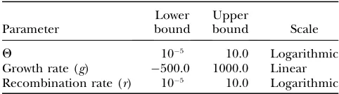
Bayesian priors for the parameters are shown in Table 1. They were set deliberately broad because we expect that biologists will not be able to provide narrow priors on many of these parameters.
John Huelsenbeck (personal communication) pointed out that repeatedly testing the Bayesian sampler on data
with the same true underlying parameters is not a fully correct test. Use of the Bayesian estimator implies that we believe that the underlying parameters are randomly drawn from the prior, but we know they are not. To test whether this affected performance of the Bayesian sampler we did an additional simulation estimatingQ, drawing the underlying values ofQfrom a prior. We did not want to use the very wide prior used in our other analyses because it would generate too many invariant data sets, so we chose a logarithmic prior from 0.05 to 0.2 (meanQ0.108) or from 0.005 to 0.02 (meanQ
0.0108) and drew theQof each data set independently from that prior. These priors were chosen to have a mean
Qvery close to the conditions in Table 1, for comparison purposes. Bayesian runs on these data used the same prior used to generate the data.
Summary statistics:We measured, for each estimated parameter, the mean estimate (maximum-likelihood estimate or maximum-probability estimate), mean up-per and lower 95% credibility or support interval boundaries, and mean boundary width. We also assessed in what proportion of runs the underlying simulation value of the parameter was rejected at the 95% level. This differs from the procedure used in Kuhneret al.
(1998), where we assessed rejection of the entire set of parameters simultaneously, as our implementation of Bayesian LAMARC is not able to score such rejections.
Effective zero for recombination rate: We include cases in which the recombination rateris zero. These cases provide some difficulty of interpretation. The logarithmic prior used by Bayesian LAMARC cannot include zero, and while likelihood LAMARC can in theory return a support-interval boundary at zero, in practice numeric precision issues cause a higher value to be returned. Therefore, in assessing whether the sup-port or credibility intervals exclude zero it is helpful to use an ‘‘effective zero’’ rather than actual zero.
We defined an effective recombination rate of zero as a recombination rate at which an average-sized co-alescent genealogy of the given number of tips, with the given number of sites, would have only a 5% chance of containing even one recombination. A value ofrthat produces a genealogy with no recombinations clearly cannot be distinguished from zero (which would also produce no recombinations). The effective zero for our higher value ofQ¼0.1 was 8.83105and for our lower
TABLE 1
Priors for population parameters
Parameter
Lower bound
Upper
bound Scale
Q 105 10.0 Logarithmic
Growth rate (g) 500.0 1000.0 Linear
Recombination rate (r) 105 10.0 Logarithmic
value ofQwas 8.83104. We have interpreted intervals
including these values as including zero and intervals excluding these values as excluding zero.
When the true value lies at one boundary of the allowable values, as in this case, the appropriate test is one-tailed rather than two-tailed, so we report the lower 5% rather than the lower and upper 2.5% regions of the likelihood or posterior probability curve. (Use of an effective zero makes it formally possible that the entire interval would be below effective zero, but this was never observed. It would presumably reflect either an in-correct choice of effective zero or a program failure.)
We do not report lower bounds of the intervals when the true value is zero, as they are often arbitrary program choices rather than actually calculated bounds.
Validation of runs:There is not, and probably cannot be, a fully reliable method for detecting convergence of MCMC samplers of this kind. In addition to varying run lengths, we used the TRACER program of Rambaut
and Drummond (2003) to compute effective sample
sizes (ESS) for a subset of our Bayesian runs. Rambaut and Drummond recommend a minimum ESS of 100 for every parameter but suggest that 200 might be a safer cutoff.
RESULTS
Parameter estimates: For all combinations of un-derlying parameters we considered, Bayesian and likeli-hood analyses gave extremely similar mean parameter
estimates. Accuracy was similar to that seen in previous studies (Kuhneret al.1995, 1998, 2000a).
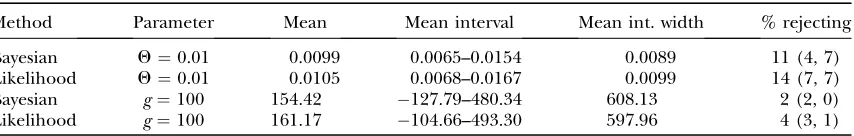
On the basis of previous results with likelihood LAMARC, we expected that the parameter estimates would be nearly unbiased in all cases considered except for growth rate, which is biased when only a few loci are analyzed (Kuhneret al.1995). This expectation was met,
with both Bayesian and likelihood analyses showing an upward bias in growth rate (Table 3). This bias is due to nonlinearity in the relationship between inferred branch length and growth rate and is not specific to Markov chain Monte Carlo analysis (Kuhneret al.1995). Support and credibility intervals: There was no consistent difference between the mean width of Bayesian credibility and likelihood support intervals, with the Bayesian intervals being wider in seven cases and the likelihood intervals wider in five cases. (We estimated the interval widths from Table 4, B and C, by assuming that their lower bounds were zero.)
An unexpected pattern was seen in how often the underlying parameter values were rejected. Some cases rejected much more often than the nominal signifi-cance level, whereas others were close to the nominal level or somewhat below it. These results were repeat-able with different data sets from similar parameter values (compare Table 2A and 2C with 2B and 2D) and with repeated analysis of the same data sets (compar-isons within Table 4A.) In general, when rejection was high for one method of analysis it was also high for the other (Figure 1).
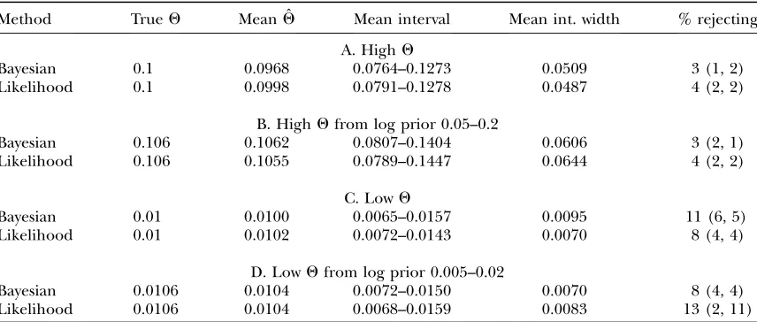
TABLE 2
Estimation ofQ
Method TrueQ Mean ˆQ Mean interval Mean int. width % rejecting
A. HighQ
Bayesian 0.1 0.0968 0.0764–0.1273 0.0509 3 (1, 2)
Likelihood 0.1 0.0998 0.0791–0.1278 0.0487 4 (2, 2)
B. HighQfrom log prior 0.05–0.2
Bayesian 0.106 0.1062 0.0807–0.1404 0.0606 3 (2, 1)
Likelihood 0.106 0.1055 0.0789–0.1447 0.0644 4 (2, 2)
C. LowQ
Bayesian 0.01 0.0100 0.0065–0.0157 0.0095 11 (6, 5)
Likelihood 0.01 0.0102 0.0072–0.0143 0.0070 8 (4, 4)
D. LowQfrom log prior 0.005–0.02
Bayesian 0.0106 0.0104 0.0072–0.0150 0.0070 8 (4, 4)
Likelihood 0.0106 0.0104 0.0068–0.0159 0.0083 13 (2, 11)
It is striking that the growth-rate estimates (Table 3), which were strongly biased upward, were nonetheless associated with rejection rates close to the nominal level. The Bayesian sampler rejected the underlying param-eter value less often than the likelihood sampler (P ¼
0.021, two-tailed binomial test). This occurred both when the rejection rate was high for both methods and when it was not and was somewhat surprising given the lack of a significant difference in interval width.
Influence of the Bayesian prior: The similarities between Bayesian and likelihood results suggested that the Bayesian prior was not strongly influencing the results, except in one case. For estimation of a recom-bination rate of 0.04 (Table 4A), the Bayesian credibility intervals were displaced downward from the likelihood support intervals, and almost all of the Bayesian method’s rejections were underestimates rather than overestimates. Examination of the curves produced by the Bayesian sampler (Figure 2) suggested that the sequence data were unable to distinguish between various low values of r, and the logarithmic-flat prior was therefore dragging the credibility intervals down-ward. However, the rate of rejection of the underlying values was still similar to that for likelihood LAMARC.
Results when the underlying values were drawn from the same prior used in the analysis (Table 2, B and D) and when the underlying values were arbitrarily fixed and a much wider analysis prior was used (Table 2, A and C) were not substantially different.
Adequacy of run lengths: We used TRACER to test the ESS of Tables 2A and 4, A (original run length) and
B. Satisfactory ESS does not guarantee convergence of the sampler, but unsatisfactory ESS strongly suggests nonconvergence. In all cases the ESS was well over the recommended cutoff. Mean and minimum ESS values are noted in the appropriate table legends.
DISCUSSION
Comparison among cases: Some parameter combi-nations showed high rejection rates in both the Bayesian and the likelihood samplers, whereas other combina-tions were consistently lower. The case withQ¼0.1 and
r ¼ 0.04 has particularly high rejection. This cannot be attributed to the high value of Q (which was well estimated on its own in Table 2, A and B) or to esti-mation ofr(as rejection rates were not elevated in Table 4B or 4C). It is not clear why some cases lead to so much higher rejection than others.
The Bayesian sampler had somewhat lower rejection in Table 4A, leading us to wonder if thex2
-approxima-tion used in the likelihood support intervals might be inaccurate (it is only asymptotically correct). We ex-plored this possibility by treating the Bayesian posterior probability curve as an estimate of the likelihood curve and applying a likelihood-ratio test (LRT) to it. If the LRT is contributing to the higher rejection rate of likelihood LAMARC, applying it to the Bayesian sampler should increase rejection. This was not found. In Table 4A, first row, the LRT rejected the underlying value ofQ
14 times (compared to 13 rejections using the 95% boundaries of the Bayesian support interval) and the underlying value of r 19 times (compared to 20). In Table 2A the LRT rejected the underlying value ofQ2 times (compared to 3). Apparently use of the LRT on the Bayesian curve produces results very similar to direct use of the support interval.
This focuses attention on inadequacy of the MCMC search as an explanation for high rejection rates. We experimented with longer searches (Table 4A) but there was little sign of improvement; however, it is possible that all of the search lengths tried were still inadequate. Use of multiple replicates did improve the rejection rate somewhat for the likelihood sampler. Replication is a longer search, but it also combines re-sults from multiple driving values, which simply length-ening the search does not.
TABLE 3
Estimation ofQand growth rate
Method Parameter Mean Mean interval Mean int. width % rejecting
Bayesian Q¼0.01 0.0099 0.0065–0.0154 0.0089 11 (4, 7)
Likelihood Q¼0.01 0.0105 0.0068–0.0167 0.0099 14 (7, 7)
Bayesian g¼100 154.42 127.79–480.34 608.13 2 (2, 0)
Likelihood g¼100 161.17 104.66–493.30 597.96 4 (3, 1)
Lengthening the search produces a better sample of ‘‘common’’ genealogies characteristic of the maximum parameter values, but if the boundaries of the credibility or support intervals are best explored by using ‘‘rare’’ genealogies, longer searches may not quickly improve the situation. The Bayesian sampler might have an advantage in that it will be able to produce rare genealogies during periods where it has accepted un-usual driving parameters (Stephens 1999), but such
periods may themselves be rare. One possible approach for likelihood LAMARC would be to run multiple replicates whose driving parameters were deliberately set near the expected 95% boundaries, in the hopes that these replicates would produce genealogies informative about the boundaries.
No signs of nonconvergence were found using TRACER, but TRACER cannot detect failure to explore
entire regions of the genealogy search space, and satis-factory ESS scores do not, therefore, guarantee a suc-cessful search.
We do not recommend the Bayesian search strategy used in this article for the analysis of individual data sets of biological interest; in the interests of speed we have not put stringent efforts into guaranteeing convergence in each analysis. A biologist with a single data set to analyze would be well advised to perform many inde-pendent searches with overdispersed random starting parameters and test that between-search variance was not significantly greater than within-search variance. If the results of this test were satisfactory, results from all searches could then be combined to give a final estimate.
Comparison between Bayesian and likelihood sam-plers:The striking general result is that the two methods
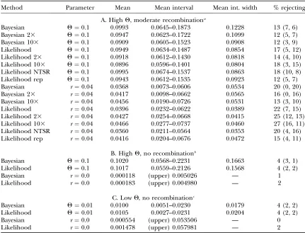
TABLE 4
Estimation ofQand recombination rate
Method Parameter Mean Mean interval Mean int. width % rejecting
A. HighQ, moderate recombinationa
Bayesian Q¼0.1 0.0993 0.0645–0.1873 0.1228 13 (7, 6)
Bayesian 23 Q¼0.1 0.0947 0.0623–0.1722 0.1099 12 (5, 7)
Bayesian 103 Q¼0.1 0.0909 0.0605–0.1523 0.0908 12 (3, 9)
Likelihood Q¼0.1 0.0949 0.0634–0.1487 0.0854 17 (5, 12)
Likelihood 23 Q¼0.1 0.0918 0.0612–0.1430 0.0818 14 (4, 10)
Likelihood 103 Q¼0.1 0.0896 0.0596–0.1401 0.0804 18 (3, 15)
Likelihood NTSR Q¼0.1 0.0995 0.0674–0.1537 0.0863 18 (10, 8)
Likelihood rep Q¼0.1 0.0943 0.0612–0.1535 0.0923 12 (5, 7)
Bayesian r¼0.04 0.0368 0.0073–0.0606 0.0534 20 (0, 20)
Bayesian 23 r¼0.04 0.0417 0.0098–0.0662 0.0565 16 (0, 16)
Bayesian 103 r¼0.04 0.0456 0.0190–0.0726 0.0531 13 (3, 10)
Likelihood r¼0.04 0.0396 0.0232–0.0622 0.0389 22 (7, 15)
Likelihood 23 r¼0.04 0.0427 0.0254–0.0668 0.0415 25 (12, 13)
Likelihood 103 r¼0.04 0.0466 0.0277–0.0737 0.0460 27 (16, 11)
Likelihood NTSR r¼0.04 0.0360 0.0211–0.0564 0.0353 20 (4, 16)
Likelihood rep r¼0.04 0.0416 0.0204–0.0676 0.0472 15 (4, 11)
B. HighQ, no recombinationb
Bayesian Q¼0.1 0.1020 0.0568–0.2231 0.1663 4 (3, 1)
Likelihood Q¼0.1 0.1017 0.0559–0.2126 0.1568 4 (2, 2)
Bayesian r¼0.0 0.000118 (upper) 0.005026 — 1
Likelihood r¼0.0 0.000183 (upper) 0.004980 — 2
C. LowQ, no recombinationc
Bayesian Q¼0.01 0.0100 0.0051–0.0230 0.0179 4 (2, 2)
Likelihood Q¼0.01 0.0105 0.0027–0.0231 0.0204 4 (2, 2)
Bayesian r¼0.0 0.000554 (upper) 0.053506 — 0
Likelihood r¼0.0 0.001478 (upper) 0.057981 — 2
Column headings are as in Table 2.
aRuns marked 23are twice as long as the original runs; runs marked 103are 10 times longer than the
orig-inals. Likelihood NTSR represents runs without use of the tree-size rearrangement step. Likelihood rep rep-resents runs where three replicates contributed to the final estimate. Mean ESSs for the original-length runs were 676 with a minimum of 214 forQand 509 with a minimum of 157 forr.
bOnly the upper boundary of the interval forris reported, and the cutoff value is 5% rather than 2.5% to
reflect the one-tailed nature of its distribution. Mean ESSs were 3486 with a minimum of 2563 forQand 4369 with a minimum of 929 forr.
cOnly the upper boundary of the interval forris reported, and the cutoff value is 5% rather than 2.5% to
performed similarly both in easy cases and in more difficult ones. The only case to show marked differences between Bayesian LAMARC and likelihood LAMARC was the high-recombination case of Table 4A, in which the Bayesian sampler characteristically produced poste-rior probability curves with long ‘‘shoulders’’ in the direction of lowr(see Figure 2 for an example) and this displaced the confidence interval boundaries down-ward. The choice of a logarithmic-scale prior that spans a wide range of indistinguishable values is the culprit here. The prior claims that the range of ln(r) values between, say,10 and9 is collectively as likely as the range of values between 5 and 4. The data can distinguish between the values in the latter case, but not in the former, resulting in a section of the posterior probability curve with no more information in it than the corresponding section of the prior curve. The net result is the frequently observed shoulder or flat section between11 and7, which, when integrated, contains a substantial part of the probability at the expense of the upper section of the curve. Use of a narrower prior would almost surely move the credibility intervals closer to the support intervals of likelihood LAMARC.
The Bayesian sampler rejected the underlying param-eter values significantly less often than the likelihood sampler, both when rejection was high and when it was low. However, because of the inclusion of both high and low cases this did not lead to a studywide advantage to the Bayesian sampler: It was closer to the nominal 5% level four times, likelihood was closer six times, and two cases were ties. We do not regard this as showing an
advantage to the likelihood sampler either, as the result clearly depended on how many of the included cases were high rejection. Bayesian LAMARC had better rejection behavior in high-rejection cases and worse in low-rejection cases. As we do not understand what leads a given case to be high or low rejection, it is difficult to generalize about the overall performance of the samplers.
Beerli(2006) finds a larger advantage for Bayesian
analysis in estimating a four-population case with 4
Q-parameters and 12 migration-rate parameters. His re-sults suggest a particular advantage to Bayesian estima-tion in dealing with cases where there is almost no power available for estimating some parameters. Further work will be needed to establish whether the differences be-tween the results of Beerli(2006) and the current study
are due mainly to the different evolutionary forces con-sidered, the much larger number of parameters in his study, or his inclusion of relatively uninformative cases. Given their similar results, the choice between the Bayesian and the likelihood sampler could invoke other qualities such as run time. The Bayesian sampler quires additional steps to vary its parameters, but re-gains some time because its curve smoothing is faster than the likelihood sampler’s multidimensional maxi-mization. In practice neither sampler had a clear speed advantage when making the same number of genealogy rearrangements. On an Athlon 20001(2 GHz, 4 MB of RAM) Linux system the runs in Table 2A (Qonly) took an average of 195 min for the likelihood sampler and 168 min for the Bayesian sampler, whereas the runs in Table 4A (Q and r) took 126 min for the likelihood sampler and 139 min for the Bayesian sampler. These results rely on the assumption that the Bayesian sam-pler requires equal numbers of parameter-change and genealogy-rearrangement steps; however, parameter-change steps are inexpensive and their frequency could be increased substantially at little time cost. We would be surprised if the amount of genealogy rearrangement needed for good estimates were to vary substantially between the Bayesian and likelihood samplers, espe-cially given that their genealogy-rearrangement accep-tance rates are similar (data not shown).
The likelihood sampler is able to compute multidi-mensional profiles while the Bayesian sampler is cur-rently limited to considering one parameter at a time, and this can lose information about correlation between parameters. While multidimensional curve smoothing is possible, it is likely to be too data hungry to succeed on short runs of the sampler. Currently, likelihood meth-ods can be recommended when information about cor-relation is required.
For implementers of new MCMC samplers, Bayesian or likelihood methods may reasonably be chosen on the basis of programming difficulty. In our hands the Bayesian algorithm was substantially easier to imple-ment. Some of its advantage may have been due to our
previous experience with the likelihood algorithm, but its curve smoothing is also more computationally ro-bust than the likelihood algorithm’s multidimensional search. However, the relative ease of implementation is likely to vary with the problem domain.
For users of MCMC programs, this study suggests that the Bayesian and likelihood approaches are similar and either one can reasonably be chosen if both are available. Agreement of results between Bayesian and likelihood analysis is not, unfortunately, evidence of correctness as the methods appear strongly correlated. It is probably best to make extensive runs with one algorithm rather than shorter runs with both.
Validity of comparing likelihood LAMARC and Bayes-ian LAMARC:Other than the differences described in
methods, Bayesian LAMARC and likelihood LAMARC
represent a single unified code base, using the same models for genealogy rearrangement and data likeli-hood evaluation and the same formulas for the co-alescent priors for each evolutionary force. Therefore, their results should be readily comparable.
Points on which the two methods differ, which should be considered in interpreting their results, include choices specific to one model or the other. The Bayesian approach requires the experimenter to choose appro-priate priors. The likelihood approach requires the experimenter to choose initial driving values and the frequency with which driving values are reconsidered. In a Bayesian run, effort must be allocated between ge-nealogy changes and parameter changes. These choices could influence the results of comparing the two meth-ods. For example, if our run conditions were optimal for one algorithm and not for the other, the results could be misleading.
Likelihood LAMARC uses its collected genealogies to evaluate the multidimensional likelihood surface and find the maximum. When this surface has a trouble-some shape (particularly likely, in our experience, when estimating growth rate) the maximization routines may not find the true global maximum. Bayesian LAMARC substitutes a single-dimensional curve-smoothing pro-cess, so is vulnerable to a different class of problems. If it does not smooth enough it may falsely select a jagged point as its maximum. If it smoothes too aggressively it may smooth away a genuine but narrow peak. Thus, differences between the methods could be due to dif-ferences in the way they form their final estimates, even if they are both effectively traversing the same search space.
Likelihood LAMARC computes a maximum-likeli-hood estimate of the best parameter values. Approxi-mate support intervals are constructed on the basis of the shape of the likelihood curve and assume that ax2
-approximation is valid, which is only asymptotically correct. Bayesian LAMARC computes a most probable estimate (the mode of the distribution of sampled parameters, after smoothing) and uses the posterior
probabilities to construct credibility intervals. While we have treated the likelihood-based and Bayesian interval information as directly comparable, the two methods are answering different statistical questions. Experience with Bayesian phylogeny estimators shows that the cred-ibility intervals do not always agree with estimates of confidence obtained in other ways, such as by boot-strapping (see, for example, Alfaroet al. 2003). This
should be kept in mind when reading and interpreting our results.
Motivation for the Bayesian sampler: A theoretical advantage of the Bayesian sampler is that it can cover search space more extensively because it is not limited to a single driving value. While the likelihood sampler considers a new driving value for each chain, within a chain it uses a single driving value to guide its sampling. Stephens(1999) has shown that this can lead to biased
support intervals. This is not a problem simply of using a poor driving value, but of using genealogies sampled at one parameter value to evaluate the likelihood at a far-distant parameter value for which they may be un-informative. The Bayesian sampler considers a range of driving values throughout its run and combines in-formation from all of them into its estimates, and this offers a theoretical advantage, especially in construction of credibility intervals.
However, if this advantage exists, it was not dramatic in our study. The most striking result was the great similarity between Bayesian and likelihood results, showing that the two methods are clearly exploring the same underlying probability surface and are both encountering difficulties with the same cases.
We thank the LAMARC team, including Joe Felsenstein, Peter Beerli, Jon Yamato, Eric Rynes, and Elizabeth Walkup, for making this project possible. We thank Richard Hudson and Jennifer Williams for providing data-simulation code and the Mathematical Biosciences Institute at Ohio State University for supporting M.K.’s attendance at a meeting where preliminary results from this study were discussed. Two anonymous reviewers provided helpful input on testing Bayesian convergence. This work was supported by National Institutes of Health grant 5R01GM51929-11 (to M.K.)
LITERATURE CITED
Alfaro, M. E., S. Zollerand F. Lutzoni, 2003 Bayes or bootstrap?
A simulation study comparing the performance of Bayesian Mar-kov chain Monte Carlo sampling and bootstrapping in assessing phylogenetic confidence. Mol. Biol. Evol.20:255–266. Bahlo, M., and R. C. Griffiths, 2000 Inference from gene trees in
a subdivided population. Theor. Popul. Biol.57:79–95. Beerli, P., 2006 Comparison of Bayesian and maximum-likelihood
inference of population genetic parameters. Bioinformatics22:
341–345.
Beerli, P., and J. Felsenstein, 1999 Maximum likelihood estimation
of migration rates and effective population numbers in two pop-ulations using a coalescent approach. Genetics152:763–773. Beerli, P., and J. Felsenstein, 2001 Maximum likelihood
estima-tion of a migraestima-tion matrix and effective populaestima-tion sizes inn sub-populations by using a coalescent approach. Proc. Natl. Acad. Sci. USA98:4563–4568.
Drummond, A. J., G. K. Nicholls, A. G. Rodrigoand W. Solomon,
genealogy simultaneously from temporally spaced sequence data. Genetics161:1307–1320.
Geyer, C. J., 1991a Markov chain Monte Carlo maximum
likeli-hood, pp. 156–163 inComputing Science and Statistics: Proceedings of the 23rd Symposium on the Interface, edited by E. M. Keramidas.
Interface Foundation, Fairfax Station, VA.
Geyer, C. J., 1991b Estimating normalizing constants and
reweight-ing mixtures in Markov chain Monte Carlo. Technical Report No. 568. School of Statistics, University of Minnesota, Minneapolis. Griffiths, R. C., and P. Marjoram, 1996 Ancestral inference from
samples of DNA sequences with recombination. J. Comput. Biol.
3:479–502.
Griffiths, R. C., and S. Tavare´, 1993 Sampling theory for neutral
alleles in a varying environment. Proc. R. Soc. Lond. Ser. B344:
403–410.
Hastings, W. K., 1970 Monte Carlo sampling methods using
Mar-kov chains and their applications. Biometrika57:97–109. Hudson, R. R., 2002 Generating samples under a Wright-Fisher
neutral model of genetic variations. Bioinformatics18:337–338. Kaplan, N., R. R. Hudsonand M. Iizuka, 1991 The coalescent
pro-cess in models with selection, recombination, and geographic subdivision. Genet. Res.57:83–91.
Kimura, M., 1980 A simple model for estimating evolutionary rates
of base substitutions through comparative studies of nucleotide sequences. J. Mol. Evol.16:111–120.
Kingman, J. F. C., 1982a The coalescent. Stoch. Proc. Appl.13:235–
248.
Kingman, J. F. C., 1982b On the genealogy of large populations.
J. Appl. Probab.19A:27–43.
Kuhner, M. K., and J. Felsenstein, 2000 Sampling among
haplo-type resolutions in a coalescent-based genealogy sampler. Genet. Epidemiol.19(Suppl. 1): S15–S21.
Kuhner, M. K., J. Yamato and J. Felsenstein, 1995 Estimating
effective population size and mutation rate from sequence data using Metropolis-Hastings sampling. Genetics 140: 1421– 1430.
Kuhner, M. K., J. Yamatoand J. Felsenstein, 1998 Maximum
likeli-hood estimates of population growth rates based on the coales-cent. Genetics149:429–434.
Kuhner, M. K., J. Yamatoand J. Felsenstein, 2000 Maximum
likeli-hood estimation of recombination rates from population data. Genetics156:1393–1401.
Metropolis, N., A. W. Rosenbluth, M. N. Rosenbluth, A. H.
Tellerand E. Teller, 1953 Equations of state calculations
by fast computing machines. J. Chem. Phys.21:1087–1092. Nielsen, R., and J. Wakeley, 2001 Distinguishing migration from
isolation: a Markov chain Monte Carlo approach. Genetics
158:885–896.
Press, W. H., S. A. Teukolsky, W. T. Vetterlingand B. P. Flannery,
2002 Numerical Recipes in C11: The Art of Scientific Computing, Ed. 2. Cambridge University Press, New York.
Rambaut, A., and A. J. Drummond, 2003 Tracer v1.3 (http://evolve.
zoo.ox.ac.uk/).
Silverman, B. W., 1986 Density Estimation for Statistics and Data
Anal-ysis(Monographs on Statistics and Applied Probability, Vol. 26). Chapman & Hall, London.
Stephens, M., 1999 Problems with computational methods in
pop-ulation genetics. Bulletin of the 52nd Session of the Interna-tional Statistical Institute, Helsinki.
Watterson, G. A., 1975 On the number of segregating sites in
ge-netical models without recombination. Theor. Popul. Biol. 7:
256–276.
Communicating editor: J. Wakeley
APPENDIX A
Waiting-time terms without growth are as follows:
exp X
u
½tðuÞ tðu1ÞX
i
kiðuÞðkiðuÞ 1Þ
Qi 1kiðuÞ
X
j6¼i
Mij
2 4
3 51rsðuÞ
2 4
3 5:
With nonzero growth the term involvingQbecomes
exp X
u
X
i
kiðuÞðkiðuÞ 1Þ
Qigi
expðgitðuÞ gitðu1ÞÞ
" #
:
The point probability densities for migration and recombination are simply proportional to the appropriate rates. The point probability density, up to a constant, for a coalescence in the absence of growth is 1/Qiand in the presence of growth is
1
QiexpðgitðuÞÞ
:
In these equations,urefers to the time interval andtto the time at the rootward end of that time interval (where times start at 0 at the tips and increase toward the root).s(u) is the count of eligible recombination locations in all lineages in intervalu. Populations are indicated byi;ki(u) is the count of lineages in populationiduring intervalu.
Because time is observed only by the accumulation of mutations, the population parameters are scaled by the neutral mutation rate per sitem, which therefore cannot be estimated separately. Population parameters areQi¼4Nemfor
populationi, immigration rateMij¼mij/mindicating immigration fromitoj, exponential growth rategidefined by
the relationshipQt¼Q0exp(gtm), and recombinationr¼C/m(not allowed to vary among populations).
APPENDIX B
Posterior-likelihood curves are smoothed using a biweight kernel of the form
forabs(t),1.0. The width of the kernel is set as
2:5sn1=5;
wherenis the number of points in the data set, andsis the smaller of the interquartile distance divided by 1.34, or the standard deviation of the sampled points.
This value can be too small (for example, if all of the sampled parameters were identical). In that case, for logarithmic priors we impose a kernel width of 0.001, and for linear priors we impose a bin width equal to
10log10ðulÞ4;
whereuandlare the upper and lower bounds of the prior.
The biweight kernel was chosen because it is bounded (unlike a Gaussian kernel) and simple to calculate. Its drawback is that, while it is bounded, it can spread slightly beyond the bounds of the prior. This is quite notable when the maximum of the posterior distribution is very close to one bound of the prior. A strictly constrained kernel might provide better results at the cost of increased computational complexity.
The formula for the kernel width is given by Silverman(1986) under the assumption that the function to be
estimated is Gaussian:
hopt¼2:78sn1=5: