ABSTRACT
MOU, GANG. Modeling and Control of a Magnetostrictive System for High Precision Actuation at a Particular Frequency. (Under the direction of Dr. Paul I. Ro.)
A magnetostrictive actuator made of Terfenol-D alloy can generate high mechanical strains with broadband response and provide accurate positioning. These characteristics have been employed as controllers and vibration absorbers in industrial and heavy structural applications, such as fast tool servo systems and precision micropositioners. Full utilization of magnetostrictive transducers in these applications requires a suitable controller as well as quantification of the transducer dynamics in response to various inputs.
However, at moderate to high drive levels, the output from a magnetostrictive actuator is highly nonlinear and contains significant magnetic and magnetomechanical hysteresis. The control of this nonlinear system is a challenge. In order to simplify this problem, 50Hz is chosen as the working frequency for the actuator in the experiments since it shows near linear property at 50Hz and the approach used at 50Hz could be extended to a broader frequency range in the applications.
As a nonlinear control approach, sliding mode control can offer some ideal properties, such as insensitivity to parameter variations or uncertainties, external disturbance rejection, and fast dynamic response. In order to obtain better tracking performance and robustness, a sliding mode control algorithm is introduced into the system.
BIOGRAPHY
ACKNOWLEDGEMENTS
I would like to express my first words of gratitude to my advisor Dr. Paul I. Ro. Without his guidance, support and encouragement this thesis would have never been materialized. Apart from advising me on the research matters, he has always been a superb mentor and supporter. His respectable attitude towards scientific work and goal for excellence would be my guide for ever. I wish to thank thesis committee members Dr. Gregory D. Buckner and Dr. Fen Wu for taking the time to give advice for my research and to review this thesis. Due to their help, lots of significant technical bugs were identified and subsequently corrected. I also wish to acknowledge and thank Mr. Ken Garrard at the Precision Engineering Center (PEC) for his help on the program in this project. Without his generosity, Chapter V would not have turned out as it did. My heartful appreciation goes to Mrs. Nancy McAllister for her great help to review my thesis word by word. Thus, numerous grammar and syntax errors in my thesis were marked out and have been corrected.
with the experimental work. I wish to acknowledge the financial support for this project, provided by a grant from the National Science Foundation (NSF).
TABLE OF CONTENTS
LIST OF FIGURES...vii
CHAPTER I: Introduction 1.1 Introduction to Magnetostriction ...1
1.2 Magnetostrictive Materials ...4
1.3 Magnetostrictive Devices ...5
1.4 Origin of the Research Project...10
1.5 Project Objectives ...11
References...13
CHAPTER II: Magnetostrictive Actuation System 2.1 The Magnetostrictive Actuation System...14
2.2 Structure of Magnetostrictive Actuator...16
2.3 Characteristics of Magnetostrictive Actuator...19
2.4 Open Loop Performance of the Magnetostrictive Actuator...26
References...32
CHAPTER III: System Identification 3.1 Modeling for the Magnetostrictive Actuator ...33
3.2 Least Squares Technique ...37
3.3 Time-Delay Model For the Magnetostrictive Actuator...39
3.4 Second order Dynamic Model for the Magnetostrictive Actuator...41
References...45
4.2 PID Controller Design ...49
4.3 Observer Design...59
4.4 Sliding Mode Controller Design...62
4.5 Sliding Mode Control with Variable Switching Gain ...69
References...74
CHAPTER V: Experiments and Analysis 5.1 Experimental Setup and Sensor Calibration ...76
5.2 Control Experiments Implementation ...80
5.3 Experimental Results and Analysis ...81
References...91
CHAPTER VI: Discussion and Future Work...93
6.1 Discussion...93
6.2 Future Work ...94
References...96
Appendices 1. Data Acquisition Program... 97
LIST OF FIGURES
Chapter I Page
Figure 1.1: Fundamental Principle of a Smart Structure Actuator………...2
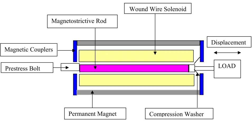
Figure 1.2: Structure of a Linear Magnetostrictive Actuator………...6
Figure 1.3: Micro-strain vs. Applied Magnetic Field……….…9
Chapter II
Figure 2.1: The Main Components of the Magnetostrictive Actuation System…………14
Figure 2.2: Cross Section of the Magnetostrictive Actuator……….17
Figure 2.3: Cross Section of the TERFENOL-D Rod………..…….18
Figure 2.4: Frequency Response of a AA-140J013 Magnetostrictive Actuator………...20
Figure 2.5: Quasi-Static Strain vs. Applied Magnetic Field H for a TERFNOL-D
Actuator……….………….23
Figure 2.6: Magnetostrictive Hysteresis under DC Voltage Inputs………...24
Figure 2.7: Magnetostrictive Hysteresis under AC Signal Input………...24
Figure 2.8: Open Loop performance with Sine Wave Input (Frequency: 100Hz,
Amplitude: 2V………..….27
Figure 2.9: Open Loop performance with Sine Wave Input (Frequency: 100Hz,
Amplitude: 3V) ……….……….………...27
Figure 2.10: Open Loop Performance with Sine Wave Input (Frequency: 50Hz,
Amplitude: 3V) ……….28
Figure 2.11: Open Loop Performance with Sine Wave Input (Frequency: 50Hz,
Figure 2.12: Open Loop Performance with Sine Wave Input (Frequency: 50Hz,
Amplitude: 10V) ……….………...…………29
Figure 2.13: Open Loop Response with Triangle Wave Input (Frequency: 20Hz, Amplitude: 1V)………..….30
Figure 2.14: Open Loop Response with Triangle Wave Input (Frequency: 50Hz, Amplitude: 1V) ………31
Chapter III Figure 3.1: Magnetostriction M vs. Applied Magnetic Field H…...……….34
Figure 3.2: Model simulated output vs. Actual output………..40
Figure 3.3: Model simulated output vs. Actual output ……….41
Figure 3.4: Model Simulated Output vs. Actual Output………44
Chapter IV Figure 4.1 Close-loop Control Experiment Block Diagram………..49
Figure 4.2: Structure of the PID Controller………..51
Figure 4.3: PID Control Simulated Diagram Using Time-Delay Model………...…53
Figure 4.4: Simulated Results using PID Controller……….54
Figure 4.5: Simulated Tracking Performance Using PID Controller………....55
Figure 4.6: PID Control Simulation Diagram Using Second Order Dynamic Model…...56
Figure 4.7: Structure of the Second Order Dynamic Model………...56
Figure 4.8: Simulated Tracking Performance Using PID Controller………57
Figure 4.9: Simulated Tracking Performance Using PID Controller………57
Figure 4.10: Simulated Tracking Performance Using PID Controller………..58
Figure 4.12: Block Diagram for the States Observer……….60
Figure 4.13 Structure of the States Observer……….62
Figure 4.14: The Concept of Sliding Model Control Approach………63
Figure 4.15: Sliding Mode Controller Block Diagram………..67
Figure 4.16: Tracking Performance Using Sliding Mode Controller and Second Order Dynamic Model (Switching Gain K = 2)………..67
Figure 4.17: Tracking Error Using Sliding Mode Control and Second Order Dynamic Model……….………...68
Figure 4.18: Tracking Error Using Pure Equivalent Control (K = 0.0)……….……69
Chapter V Figure 5.1: Optical Sensor and Magnetostrictive Actuator with Clamps………. 77
Figure 5.2: Sensor Calibration Experiment Setup……….78
Figure 5.3: Angstrom Resolver Sensor Probe Calibration Curve………..79
Figure 5.4: Schematic Diagram of the Experimental Setup………..80
Figure 5.5: Open-loop Performance of the Actuator……… 81
Figure 5.6: Close loop control using PID controller……… 82
Figure 5.7: Close loop output vs. desired output………...82
Figure 5.8: PID control output………...83
Figure 5.9: PID control output……….. 83
Figure 5.10: PID control output vs. Desired Trajectory………84
Figure 5.11: PID controlled output vs. Desired Trajectory………...84
Figure 5.12: Tracking Error using PID control………..85
Figure 5.14: Experiments result using Sliding Mode Controller…...86
Figure 5.15: Sliding Mode Controller Response ………..87
Figure 5.16: Desired Trajectory vs. Trajectory using Sliding Mode Controller…………88
Chapter I
Introduction
1.1 Introduction to Magnetostriction
In mechanical and manufacturing industries, smart materials have been widely used to obtain high precision actuation and controlled response trajectory. Over the past decades, with advances in material sciences and actuation technologies for high precision purposes, the demand for the design and control of high precision actuators of smart structures, such as piezoelectric, electrostatic and magnetostrictive actuators, has grown quite noticeably.
Input Energy - Power
Input Energy- Output Energy-
Control Mechanical Work
Figure 1.1: Fundamental Principle of a Smart Structure Actuator
Among these smart materials, piezoelectric material is known for providing some ideal properties. For instance, it can generate actuation with very high resolution and operates under high frequency range and low voltage. Therefore, piezoelectric actuators (PZT) have been applied widely in industry. However, in the circumstances of low frequency range and higher loading bearing, piezoelectric material does not show those consistent performances. Traditional actuators, such as hydraulic and piezoelectric actuators are usually not suitable to control the motion of cutting tools due to the limitation of either the bandwidth or the actuating force. Magnetostrictive material exhibits high force at nearly instantaneous speed; and actuators made of these materials occupy a small volume and require relatively low voltage input. Magnetostrictive material has great potential to perform better than piezoelectric devices and hydraulic systems in machining applications. It next emerged as an ideal material for high precision actuation and sensing. And, with the progress in the development of magnetostrictive materials and alloys, magnetostrictive actuators have even broader applications.
Magnetostrictive material is a compositive alloy containing terbium (Tb) and dysprosium (Dy) with iron (Fe). Terbium (Tb) generates strains; dysprosium (Dy)
minimizes the field strengths required to generate the strains; iron (Fe) allows the alloy’s exceptional transduction properties to be used at or above room temperature. Terfenol-D is the best known alloy with the typical composition Tb0.3Dy0.7Fe1.95. The name Terfenol-D comes from its metallic elements: TER ~ terbium, FE ~ iron, NOL ~ Naval Ordinance Labs (now NOWC), where the material was first developed, and D ~ dysprosium. While the Terfenol-D devices require low voltage level input, Terfenol-D can produce "giant" magnetostriction, a strain greater than most available commercial smart materials.
There exist two types of magnetostriction. The first one is called spontaneous magnetostriction. If a magnetostrictive material is cooled from Curie points, the magnetostrictive material will go through a transition from state of paramagnetism to the state of ferromagnetism. The procedure forms spontaneous magnetostriction. The second type is field-induced bulk magnetostriction. It is described as a property encountered in magnetic materials where the material changes its shape upon the application of a magnetic field. The magnetostriction discussed in this thesis refers to the field-induced bulk magnetostriction. Magnetostrictive materials have the ability to convert magnetic energy into mechanical energy and vice versa. As a magnetostrictive material is magnetized, it strains or exhibits a fractional change in length accompanied by an inverse change in girth. Conversely, if an external force is applied to cause a strain, the magnetic state of the material changes. This magnetostriction is quantifiable and often defined using the following equation:
L L ∆ =
where ∆L represents the changes measured in length, L is the constrained length of the magnetostrictive rod of the actuator. For a Terfenol-D actuator, the value of λ is often at the range of 1500-2000 parts per million (ppm). In contrast, the value of λ is only 20 ppm for iron. Therefore, the value of λ is the indicator of the level of magnetostriction. Apparently,λ is of the same unit with strainε. For magnetostrictive actuators, the total strain ε consists of λ and the elastic deformation.
This coupling process between magnetic and mechanical energies is the transduction capability that allows a magnetostrictive material to be used in both actuation and sensing devices.
1.2 Magnetostrictive Materials
Magnetostrictive materials have been studied for a long time. In 1842, James Joule identified the very first magnetostrictive effect when he observed that a sample of nickel changed in length while being magnetized. Subsequently, cobalt, iron and alloys of these materials were found to show a significant magnetostrictive effect with strains of about 50ppm.
In the 1960s, the rare-earth elements terbium (Tb) and dysprosium (Dy) were found to have between 100 and 10,000 times the magnetostrictive strains found in nickel alloys. However, these properties only exist at very low temperature. Desired actuation applications operating at ambient temperature and above were almost impossible.
Since then, researchers have looked for a material that would operate at a high temperature and have a large magnetostrictive strain, but would require only a low magnetic field. It is found that the addition of iron to Tb and Dy to form the compounds TbFe2 and DyFe2 brought the magnetostrictive properties to room temperature. These materials also required very large magnetic fields to generate large strains. By alloying the two compounds, the magnetic field required to produce saturated strains was considerably reduced. The resulting alloy Tb.27 Dy.73 Fe1.95, commercially known as Terfenol-D, is at present the most widely used magnetostrictive material. Terfenol-D is capable of having strains as high as 2000-3000 ppm [1]. And since the 1980s, it has been a commercially available material for application in many areas.
1.3
Magnetostrictive Devices
Concerning the classification of magnetostrictive devices, there are various categories, either based on the operating frequency or applications. For convenience, magnetostrictive devices are grouped into five main categories:
1. Mechanical magnetostrictive actuators
and rotational actuators are two main sub-categories, based on the type of motion the actuators provide.
Figure 1.2: Structure of a Linear Magnetostrictive Actuator
Figure 1.2 shows the structure of a linear actuator. With the proper control algorithm, this actuator could be applied as a fast tool servo driven system, which is specifically designed for turning non-round parts. For example, Active Machining System (AMS), made by Etrema Inc., is such a computer controlled system that utilizes the power and fast response of a magnetostrictive actuator to precisely position the cutting tool in synchrony with a machine tool spindle. The actuator, applied as a fast tool servo, is mounted on the cross-slide of a lathe and controls the position of the cutting tool, according to control commands from the computer.
2. Sonar devices at low frequency
LOAD Prestress Bolt
Magnetic Couplers
Magnetostrictive Rod
Wound Wire Solenoid
Permanent Magnet
Displacement
Magnetostrictive actuators are often operated at low frequency in this category. One typical application is the underwater acoustic sonar. Terfenol-D has been proven very attractive for underwater sound projection given its output strain, force and impedence-matching characteristics. Searching for more powerful sonar units forced researchers to increase either the size of the radiating surface or the vibration amplitude of the devices. On the other hand, the volume and weight constraints typically limit the allowable size of the device. Therefore, the research was focused on improving the vibration amplitudes. This demand led to the reviving of the flextensional transducer. Magnetostrictive flextensional transducers provide high power at low frequencies. The power output of the magnetostrictive flextensional transducers is about 25 times greater than that of PZT flextensional transducers. This occurs because its dynamics strain is approximately five times larger, and the power output is approximately proportional to the square of the strain.
3. Shock and vibration isolation devices
In conventional vibration isolation systems, spring and damper are often not effective in low frequency range and large mass cases. With the introduction of magnetostrictive actuators, active and passive vibration cancellation methods become very appealing. A feedback control system is often employed with suitable transducers to sense displacement, velocity and acceleration. Thus it can reduce the shock or vibration effectively.
Although piezoelectric actuators are sometimes preferred for ultrasonic or even megahertz range ultrasonic, the ruggedness and durability of magnetostrictive devices constitute a very appealing characteristic. In addition, magnetostrictive materials do not need to be repolarized when accidently heated beyond the Curie temperature point, whereas the piezoelectric actuators require this.
The ultrasonic magnetostrictive actuators are used in the fields of sonochemistry, ultrasonic welding, food processing, waste material conversion and ultrasonic machining.
Chemical processes such as polymerization can be commercialized using Terfenol-D ultrasonics. Several processes for ultrasonic destruction of environmentally damaging materials are in final stages of development. Since Terfenol-D is a low voltage, current driven magnetostrictive material, hand tools can be made safer. The high energy density of Terfenol-D also makes hand tools smaller in size.
5. Miscellaneous applications
Secondly, magnetostriction is a property that causes certain ferromagnetic materials to change shape in a magnetic field. The magnetic domain in the crystal will rotate when a magnetic field is applied. This provides a proportional, positive and repeatable expansion in microseconds, which is desired for actuation.
Lastly, the magnetostriction effect arises from an alignment of the magnetic domains. The crystal's magnetic anisotropy couples the magnetic field with the lattice distortion and consequently produces strain. The magnetostrictive effect is very sensitive to composition and manufacturing.
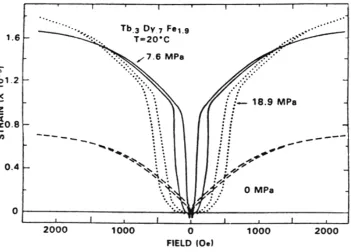
Figure 1.3: Micro-strain vs. Applied Magnetic Field
plotted as a function of the applied magnetic field. In addition to the highly nonlinear property, it exhibits hysteric responses. Given the nonlinearities, using a linear feedback control scheme is not practical. Therefore, it’s a challenge to implement real-time control for the magnetostrictive actuator.
1.4 Origin of the Research Project
Magnetostrictive actuators have various applications in mechanical area. The typical applications of the magnetostrictive actuation include a fast tool servo system for tool positioning and control in the manufacturing industry—an example is, the smart machine tools with actuators to compensate for structural vibrations under variable loads; combustion engine fuel injections in the internal combustion industry; pumps and valves in the hydraulic industry; high precision positioning in the defense and aerospace industry—an example is the smart fixed wings with actuators that alter airfoil shape to accommodate changing drag or lift conditions.
As seen above, magnetostrictive materials have some desirable properties for actuation. However, they also show a very nonlinear property. In addition, a so-called non-affine property exists within a magnetostrictive system. These properties are the main limitations for its application in industry.
nonlinear system, motivated by this, modeling and control of a magnetostrictive actuation system is chosen as the subject for this project.
The main equipment used in this research includes a Magnetostrictive Actuator (Model#: AA-140J) manufactured by Etrema Products Inc., IA; a PWM AC SERVO AMPLIFIER (Model#: 16A20ACT Brush Type) manufactured by Advanced Motion Controls, CA; an Angstrom Resolver (Model 101) assembled by Opto Acoustic Sensors at Raleigh, NC; an IBM-compatible personal computer; and a DT2823 ISA-bus DSP-board marketed by Data Translation Inc. at Marlboro, MA. The actuator and the amplifier were donated by Lord Corporation located at Cary, NC. This research project obtained its main financial support from the National Science Foundation (NSF). The research work related with this project was physically done at the Precision Engineering Center (PEC), Mechanical and Aerospace Engineering Department, North Carolina State University at Raleigh, NC.
1.5 Project Objectives
Since modeling and control for the magnetostrictive system is the objective of this project, the following related procedures, which also make up the main contents of this thesis, were necessary for the research.
Chapter II includes main contents on design and structure of the magnetostrictive actuator. It also covers the application of magnetostrictive actuators. And, it presents the characteristics of the magnetostrictive materials and the actuator, especially on the nonlinear property and hysteresis phenomenon.
In Chapter III, the system identification problem is addressed. Using Least Square Technique (LST) and SAS System V8 program, a time-delay and dynamic model is established by matching the data series gathered from the input and output signal on the actuator. It’s a so-called Black Box Model.
Chapter IV illustrates the controller design issue. PID control and sliding mode control (SMC) are two main control techniques being demonstrated. Matlab simulations are done first in order to verify the validation of the established model. The proposed controllers will demonstrate their tracking performances, respectively.
Chapter V provides the implementation of the control experiments and results analysis. Incorporated with a data acquisition board and computer, the experiments are conducted. The close loop performance of the proposed controller is to be verified by the experiments. Both results from open loop and close loop control experiments are compared and discussed.
References:
1. A P Dorey and J H Moore, “Advances in Actuators,” IOP Publishing Ltd 1995. 2. Ralph C. Smith, “A Nonlinear Model-Based Control Method for Magnetostrictive
actuators”, Proceedings of the 36th Conference on Decision & Control, December 1997.
3. Ralph C. Smith, “Inverse Compensation for Ferromagnetic Hysteresis,” Proceedings of the 38th Conference on Decision & Control, December 1999.
4. M. E. H. Benbouzid, “Artificial Neural Networks for Finite Element Modeling of Giant Magnetostrictive Devices,” IEEE Transaction On Magnetics, Vol. 34, No. 6, November 1998.
5. L. Gros, G. Reyne, C Body and G. Meunier, “Strong Coupling Magneto Mechanical Methods Applied to Model Heavy Magnetostrictive Actuators,” IEEE Transaction On Magnetics, Vol. 34, No. 5, September 1998.
6. R. Venkataraman, “Modeling and Adaptive Control of Magnetostrictive Actuators,” Ph.D Dissertation, University of Maryland, College Park, 1999.
7. Ralph C. Smith, “A Nonlinear Physic-Based Optimal Control Method for Magnetostrictive Actuators,” ICASE Report No. 98-4.
8. R D Greenough, “Actuation with Terfenol-D,” IEEE Transaction on Magnetics, Vol. 27, No. 6, November 1991.
9. Gutierrez, H. M. and Ro, P. I., "Sliding-mode control of a nonlinear-input system: application to a magnetically levitated fast-tool servo", IEEE Trans. on Ind. Elec., vol.45, no.6, pp. 921-927, 1998.
Chapter II
Magnetostrictive Actuation System
2.1 The Magnetostrictive Actuation System
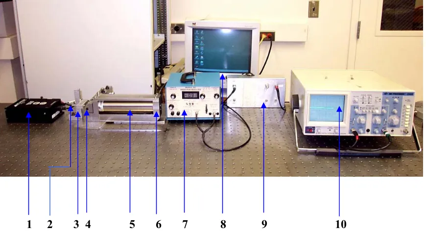
1 2 3 4 5 6 7 8 9 10
Figure 2.1: The Main Components of the Magnetostrictive Actuation System
As demonstrated in Figure 2.1, the magnetostrictive actuation system in this
research project is made of the following components:
1. Brush type PWM servo amplifier, manufactured by Advanced Motion Controls,
Camarillo, CA. Pulse width modulation (PWM) is the most efficient and cost-effective
approach for amplifying the electric signals in a precision motion control application. The
high-energy signal. This PWM amplifier has several operation modes to select from: current
mode, voltage mode, IR compensation mode, and tachometer mode. Since a DT2823
DSP board is employed in this system and its output is a voltage signal, the voltage mode
is selected as the operation mode.
2. Optical sensor, produced by Opto Acoustic Sensors, Cary, NC
3. Fixture, used to hold the Optical sensor probe.
4. Cutting tool, mounted on the actuator clamp, provided by Lord Corporation, Cary, NC.
5. Magnetostrictive actuator, manufactured by Etrema Products Inc. in Ames, IA.
6. Angstrom Resolver, with filter and signal processing circuits inside for receiving the
signal from the optical sensor.
7. Personal Computer, to execute the control program and store collected data.
8. AD/DA converter board and its interface box, made by Data Translation Inc. at
Marlboro, MA—used to collect data and generate control commands.
9. Fixture, clamp plates and attached structure, machined by Lord Corporation, Cary,
NC. In order to get higher precision and keep the actuator from free vibration movement
caused by the actuation, the actuator itself needs to be fixed on the desktop table.
10. Oscilloscope, used to observe the signals in and out from the actuator.
This magnetostrictive actuator, incorporated with the other components, is also a fast
tool servo system, capable of generating high precision actuation movement. A typical
application is cutting work pieces with irregular shaped profiles. For instance, with a
proper controller, the actuator can be mounted on a diamond turning machine (DTM) to
2.2 Structure of the Magnetostrictive Actuator
The actuator model in this research project is an AA–140J013ES1 magnetostrictive
Terfenol-D actuator manufactured by Etrema Products Inc. in Ames, IA. It’s a linear
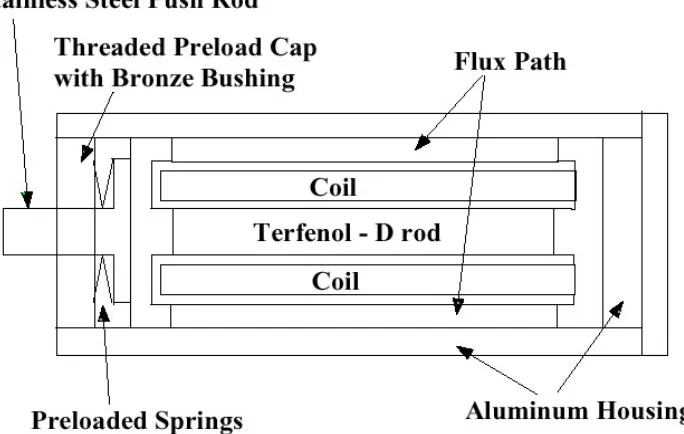
actuator with an actuation range up to 200 micrometers. Figure 2.2 illustrates the main
structures of this magnetostrictive actuator along its cross-section. The following
components comprise the magnetostrictive actuator:
1. A rod made of a smart material alloy named Terfenol-D, which converts electrical
inputs (current or voltage) into mechanical outputs.
2. A nonlinear preload spring, which provides the prestress. An optimized prestress
system will optimize the output and efficiency of the actuator, especially for low
load applications. The prestress is determined by the selected compliance and
time constant of the springs.
3. A cylindrical permanent magnet. This component provides a magnetic field bias
Hb for the actuator that is able to reduce power consumption, minimize the need
for DC bias current, and minimize heat generation. In addition, magnetic bias is
necessary in order to get approximate linear response in its displacement.
4. A wound wire solenoid (coils), with current or voltage input, provides the
actuation power through magnetic flux.
5. A stainless steel push rod, the main moving part within the actuator. It is the
executive mechanism of the actuation for the linear axial displacement.
6. A non-magnetic outer housing, which is often made from aluminum. This part
Figure 2.2: Cross Section of the Magnetostrictive Actuator
If a magnetic field is applied (the deformation of the actuator in response to
external stimulus as a change in the applied magnetic field) the result is a motion of the
push rod with respect to the outer casing. This motion is along its axial direction and is
utilized for high precision actuation purposes.
This actuator incorporates a permanent magnet bias and preloaded springs for
prestress. The unit length is 22.0 cm and the unit diameter is 4.7 cm. The housing is made
of aluminum while the push rod, i.e. the moving unit, is made of stainless steel. The
prestress is adjustable from 0 to 1 KSI (kilopounds per square inch, 1 KSI = 6.9 MPa).
Figure 2.3: Cross Section of the TERFENOL-D Rod
(Courtesy of ETREMA Products, Inc)
Figure 2.3 gives the dimension and size of the Terfenol-D rod in the actuator. The
following table lists the dimension parameters of the magnetostrictive actuator.
Model#: AA-140J013
Diameter D: 47.0 mm (1.85”)
Length L1: 198 mm (7.80”)
Length L2: 220 mm (8.68”)
Connector Center B: 19 mm (0.76”)
Flat Width FW: 7.9 mm (0.31”)
Flat Length FL: 6.4 mm (0.25”)
Thread T1 and T2 in English: 3/8-24 UN 2B 0.53 Deep; 3/8-24 UN 2A 0.50 Long
Thread T1 and T2 in Metric: M8 x 1.25-11 mm Deep; M8 x 1.25-12 mm Long
Unit Weight: 2.3 kg (5.07 lb)
Table 2.1 Dimension parameters of Magnetostrictive Actuator (AA-140J013)
As illustrated in Figure 2.2, the magnetostrictive rod made of Terfenol-D material
is the main component of a magnetostrictive actuator. Magnetostrictive material provides
many desirable properties for the magnetostrictive actuator. The most important
characteristics are:
1. Larger displacement
For accurate positioning of mechanical loads, with unsurpassed force and speed,
Terfenol-D shows outstanding capabilities among the various solid-state actuators. For
the voltage signal input under the same amplitude and frequency, magnetostrictive
material performs a longer displacement than most of the other commercial smart
materials such as piezoceramics or nickel alloys. This property is especially appealing for
the application of long-range actuation.
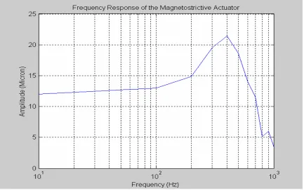
2. Frequency response
The magnetostrictive actuator could operate over a large frequecy range from DC to
20 KHz. This brings a broad application from low-frequency range to ultrasonic range.
As seen in Figure 2.4, the near linear range is about 20Hz to 200Hz.
The frequency response of an actuator is determined not only by the inherent
properties, for instance, inductance and speed, of the magnetostrictive material, but is
strongly influenced by the mechanics of the system, namely, the physical construction of
the device and its Q factor and the inertial effect of the whole system. The design of the
outer housing structure also has an influence. Due to the existence of macroscopic eddy
limitation can be minimized by laminating the Terfenol-D material. Its working
frequency range thus could be extended to 80 kHz range if the thickness of lamination is
in 1 mm range, as predicted by Etrema Products Inc.
Figure 2.4: Frequency Response of AA-140J013 Magnetostrictive Actuator
3. High strain
For actuators, high strain means larger actuation movement and bigger load. With the
development of the magnetostrictive materials, the strain goes up steadily to 2000-3000
ppm range, much higher than those of other commercial smart materials.
For a magnetostrictive actuator, the concept of precision is related to its actuation
range and repeatability. A magnetostrictive actuator can provide repeatable displacement
with high accuracy, ideal for high precision purpose acutation. A Terfenol-D rod with
10cm length and 5 cm2 could have a minimum step of the change in length of 0.01 nm
within its linear displacement of 100 micrometers [10].
5. Operating under low voltages
Compared with other smart structure actuators, such as piezoelectric crystals, which
require higher voltages (200-300 Volts) to produce desired mechanical deformations,
magnetostrictive materials readily respond to significantly lower voltages, often around
10-50 Volts. A DSP board can provide the input signal in this range with a moderate
amplifier.
6. Fast response
The mechanical response time of a magnetostrictive actuator is within several
microseconds due to the molecular level of the magnetostrictive strain. For example,
under a 20Hz AC signal, the response time is about 0.3 microseconds. Fast response is
crucial for high precision actuation, since it will reduce the tracking error within a short
time period. And fast response is particularly good for the implementation of a real-time
controller.
Although a magnetostrictive actuator is senstive to temperature variation, it can
operate over a wide temperature range from 40 to 200 °F. In order to get ideal
performance with maximum strain, room temperature is required. Strain under other
temperature conditions will cause a strain decrease.
2.3.1 Magnetostriction Hysteresis
In addition to the ideal properties, magnetostrictive material shows strong hysteresis.
The magnetostrictive actuator shows a strong hysteretic relationship between the current
or voltage input and its actuation displacement.
Hysteresis, in Greek, means lag behind.Apparently, this hysteresis phenomenon is
partly due to the lag of the response between the input and output. In view of energy, this
magnetostrictive hysteresis phenomenon is caused by the energy dissipation within the
system.
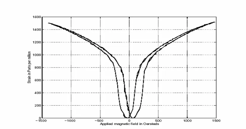
Figure 2.5 describes the association of quasi-static strain and applied magnetic field
H. A very small linear part around the origin point, the apparent different paths in Figure
Figure 2.5: Quasi-Static Strain vs. Applied Magnetic Field H for an
TERFNOL-D Actuator (Courtesy of ETREMA Products, Inc)
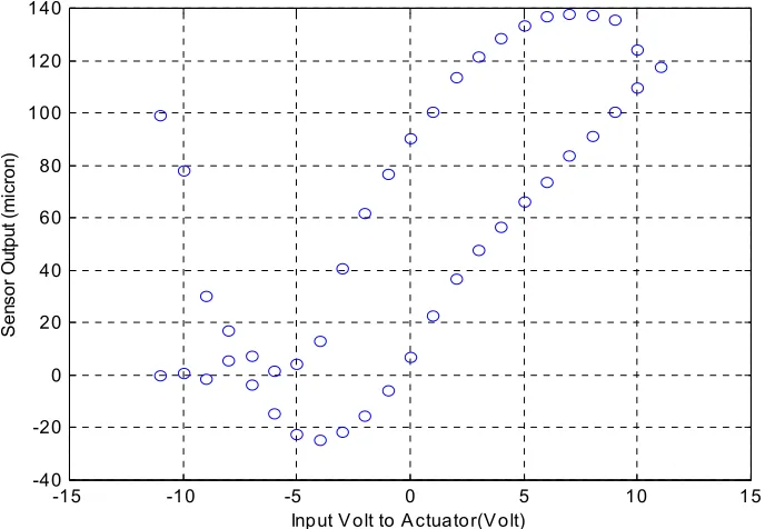
The values of each point in Figure 2.6 are obtained by inputing the DC voltage to the
acuator and measuring the corresponding displacement. The input voltage goes up
gradually from -11V to 11V, inceremented by 1V each step. Then voltage input goes
down from 11V, step by step, and back to -11V DC again. The waiting time between two
consecutive voltage inputs is about 1 minute. Apparently, even when the input voltages
are the same at the up and down procedure, respectively, the corresponding
displacements of the actuator are different. This difference in amplitudes in Figure 2.6
can reach as large as 100 micrometers. This property is called magnetostrictive
Figure 2.6: Magnetostrictive Hysteresis under DC Voltage Inputs
Figure 2.7: Magnetostrictive Hysteresis under AC Signal Input
Hysteresis is an important property of the magnetostrictive actuator. Likewise,
under the inputs of an AC voltage signal, the magnetostrictive actuator shows hysteresis,
although it’s somewhat different. The above Figure 2.7 shows the magnetostrictive
hysteresis. Obviously, under AC signal inputs, the energy loss is larger than those under
-15 -10 -5 0 5 10 15
-40 -20 0 20 40 60 80 100 120 140
Input V olt to A ctuator(V olt)
S
e
ns
o
r O
ut
put
(
m
ic
ro
DC signal inputs. Roughly, the amplitude of the displacement of the actuator on the
upward path is proportional to the amplitude of the input signal, whereas the downward
path is not. Instead, it shows a steep jump midway in its path back to the origin point.
2.3.2 Nonlinearities and Non-affine Property
In most cases, a linear range is required for actuation application. However, the
magnetostrictive material shows strong nonlinearities. The behavior of a
magnetostrictive actuator is nonlinear in every aspect. First, with an applied magnetic
field, the magnetostrictive core will be magnetized nonlinearly. In other words, the
magnetostriction is not proportional to the magnetization. The prestress mechanism
inside the magnetostrictive actuator causes nonlinearities as well. Washers are usually
used in this prestress mechanism against the magnetostrictive core. When compressed to
some extent, they produce nonlinearities and thus bring mechanical hysteresis to the
actuator. If the control input is coupled nonlinearly with states and can’t be decoupled
through analytical methods, this system is called a non-affine system.
Due to the existence of nonlinearities, the actuation displacement is expected to be
not proportional to the amplitude of the input signal. A proper controller is essential for
its application in manufacturing.
2.3.3 Temperature effects
caused by changing temperature. The thermal expansion ratio of the magnetostrictive
core is about 12Χ10−6/oC. Roughly, when heated from room temperature (20oC) to 100oC, the thermal expansion could reach 1.5% of the whole length of the Terfenol-D
rod. That’s up to 0.003m, which is not an allowable elongation for a 0.2m long actuator.
However, the displacement of the actuation motion will be smaller, since the strain of the
magnetostrictive core will decrease dramatically as the temperature increases. As a result,
the total changing in the displacement is the combination of these factors.
Therefore, maintaining a controlled room temperature is critical in applications.
Certain cooling methods are necessary for the operation. For instance, in order to cool off
the magnetostrictive actuator in operation, a certain time waiting (at least 15 minutes) is
kept between two consecutive experiments. In high precision applications, heat sink and
cooling fluid are required to maintain the required temperature.
2.4 Open Loop Performance of the Magnetostrictive Actuator
In the experiments, voltage signals with different frequencies and different
amplitudes are imposed on the magnetostrictive actuator in order to see how the actuator
behaves. Thus, raw data are being collected for modeling purposes. Some of the
Figure 2.8: Open Loop performance with Sine Wave Input (Frequency:
100Hz, Amplitude: 2V)
Figure 2.9: Open Loop performance with Sine Wave Input (Frequency:
100Hz, Amplitude: 3V)
actuator with input frequency of 100Hz. From Figure 2.8 to Figure 2.9, the amplitude
increases from 2 volts to 3 volts. The actuation displacement then increases from 25
microns to 150 microns, roughly. And the displacement trajectory with 2V is smoother
than those with 3V amplitude. Obviously, the actuation displacement is not proportional to
the amplitude of the input signal. In other words, it’s a nonlinear system.
Figure 2.10: Open Loop Performance with Sine Wave Input
(Frequency: 50Hz, Amplitude: 3V)
A trend that can be observed from these figures is, with lower frequency or
amplitude input, the displacement trajectory is smoother than those with higher
frequency or amplitude input. In other words, the higher the operating frequency is,
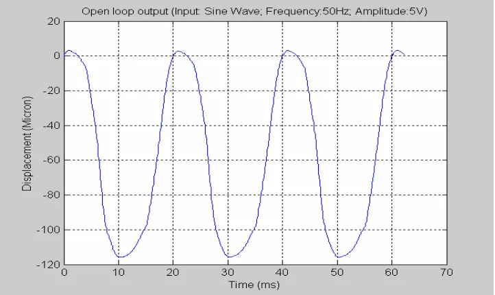
Figure 2.11: Open Loop Performance with Sine Wave Input
(Frequency: 50Hz, Amplitude: 5V)
Figure 2.12: Open Loop Performance with Sine Wave Input
(Frequency: 50Hz, Amplitude: 10V)
Figure 2.10 through Figure 2.12 also show the open loop performance under the
Here, however, the displacement is not proportional to the magnitude of the input
voltage; i.e., it is very nonlinear. This phenomenon is quite obvious, especially under
high drive level (high frequency or amplitude). Around the peaks and valleys of the
output sinusoid wave, the nonlinearity is very prominent. If the amplitude or frequency of
the input signal increases to some degree, the nonlinearity will prevail in the
performance. If no proper controller is introduced, this property will definitely limit the
application of the magnetostrictive actuator.
The following Figure 2.13 and Figure 2.14 show another open loop output under the
input of a triangular wave signal. These results verify the fact that the magnetostrictive
actuator is a very nonlinear system under various types of inputs.
Figure 2.13: Open loop response with triangle wave input
Figure 2.14: Open loop response with triangle wave input
(Frequency: 50Hz, Amplitude: 1V)
The control of this actuation system is the main interest, and then not only the
modeling of the actuator itself, but also the associated components of the actuator are
concerned. This modeling procedure is fraught with uncertain knowledge of the system
that might change with temperature and time. Without knowing the uncertainties
precisely, it’s still possible to use techniques of adaptive and robust control if a rough
knowledge of the uncertainty can be obtained. Hence, this actuation system including the
magnetostrictive actuator itself along with the associated prestress, magnetic path, and
the PWM amplifier will be modeled as a whole black box system, which is the topic of
References:
1. A P Dorey and J H Moore, “Advances in Actuators,” IOP Publishing Ltd 1995.
2. Marcelo J. Dapino, "Nonlinear and Hysteretic Magnetomechanical Model for
Magnetostrictive Transducers," PhD Dissertation, Iowa State University, 1996.
3. Ralph C. Smith, “A Nonlinear Model-Based Control Method for Magnetostrictive
actuators,” Proceedings of the 36th Conference on Decision & Control, 1997.
4. Ralph C. Smith, “Inverse Compensation for Ferromagnetic Hysteresis,”
Proceedings of the 38th Conference on Decision & Control, December 1999.
5. M. E. H. Benbouzid, “Artificial Neural Networks for Finite Element Modeling of
Giant Magnetostrictive Devices,” IEEE Transaction On Magnetics, Vol. 34, No.
6, November 1998.
6. L. Gros, G. Reyne, C Body and G. Meunier, “Strong Coupling Magneto
Mechanical Methods Applied to Model Heavy Magnetostrictive Actuators,” IEEE
Transaction On Magnetics, Vol. 34, No. 5, September 1998.
7. R. Venkataraman, “Modeling and Adaptive Control of Magnetostrictive
Actuators,” Ph.D Dissertation, University of Maryland, College Park, 1999.
8. Ralph C. Smith, “A Nonlinear Physic-Based Optimal Control Method for
Magnetostrictive Actuators,” ICASE Report No. 98-4.
9. R D Greenough, “Actuation with Terfenol-D,” IEEE Transaction On Magnetics,
Vol. 27, No. 6, November 1991.
10.Sergey F. Tsodikov, Vadim I. Rakhovsky, “Magnetostrictive Force Actuators For
Superprecise Positioning,” IEEE 18th Int. Symp. On Discharges and Electrical
Chapter III
System Identification
3.1
Modeling of the Magnetostrictive Actuation System
Due to the existence of the magnetostriction, hysteresis, and nonlinearities,
modeling of a magnetostrictive actuator is a challenging work. Researchers have tried
various methods to model magnetostrictive actuators. Most of the models for
magnetostrictive actuators are based on the H-M curve [1]; i.e. the relationship between
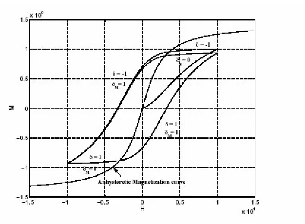
the magnetostriction M and the applied magnetic field H as shown in Figure 3.1. There are two main categories in the modeling techniques for the magnetostrictive hysteresis—
the Preisach approach [3, 4] and the quasi-macroscopic models. The Preisach model
provides an observed characterization of the relations between the input and output of the
magnetostrictive materials, but ignores some unmodeled physical mechanisms. It’s a
universal approach, in a sense. The model requires the estimation of many numerical
parameters, but does not try to include the physical dynamics of the material. The second
or quasi-macroscopic model is a physical-based model, which is also called the domain
wall approach. It concerns both the reversible and irreversible domain wall movements in
the material. And the approach uses parameters related to the magnetic characterization
of the input magnetic field. This second modeling method is formed by extending Jiles
Figure 3.1 Magnetostriction M vs. Applied Magnetic Field H
In 1983, Jiles and Atherton [5, 6] proposed a model for ferromagnetic hysteresis
with phenomenological and thermodynamic considerations. This model is very appealing
from the control point of view because it describes hysteresis as the solution of four
differential equations. Some researchers proposed a model using finite element analysis
methods. Others developed low dimensional models using the energy balance principle
[4]. Other modeling approaches concerned the development of a physics-based model for
magnetostrictive material that captures hysteretic phenomena and can be subject to
rigorous mathematical analysis towards control design [5].
The behavior of a magnetostrictive actuator, and thus its application in engineering,
depends not only on the energy type (electromagnetic, elastic, or thermal) supplied to it,
but also on how this energy is applied. In particular, the sequence of these energies
indicates the complexity of magnetostrictive behavior and the existence of coupling
between energy regimes. In order to fully utilize the desirable features of Terfenol-D, it is
necessary to characterize the electric, magnetic elastic, and thermal regimes, as well as
the interactions among them.
A proper mathematic model can accurately predict the performance of a transducer
in the form of a mathematical formulation that provides some numerical output in
response to a numerical input. Depending on the degree of accuracy, models can simulate
actuator performance or even predict it precisely. Mathematical performance simulations
are highly useful, for predicting actuator behavior is ultimately desirable.
Predictive modeling is relevant to the use of magnetostrictive actuators in three
ways. First, well-posed models provide the ability to scale results in a way that
experiments often do not. For instance, although the magnetostrictive actuator model
developed in this thesis is dependent on the actuator size and model, it is still able to
provide a modeling approach for a common magnetostrictive actuator.
Second, predictive modeling allows the actuator designer to understand and analyze
actuator behavior before any prototype is developed. Thus, time and cost to design are
Finally, in control applications, modeling can enable the knowledge of how much
change in the voltage input that is necessary to obtain a desired change in the output for
displacement.
The next question is how to predict the actuator behavior. The simplest and perhaps
most common model of magnetostrictive performance is the linear piezomagnetic
equations [6]. These equations represent the magnetic-elastic bi-directional energy
transduction in a form amenable to performance modeling, material property
characterization, electric circuit analogue representations, and control implementation.
The value, however, of this model is limited. The linear piezomagnetic equations provide
insight on the actuator performance at the low signal level, where the performance of the
magnetostrictive actuator is quasi-linear. Magnetostrictive transduction is an intrinsically
nonlinear and hysteretic process; thus, the modeling procedure should address the
nonlinear regimes properly found in applications.
Therefore, a new approach to modeling a magnetostrictive actuator will be
proposed based on statistical principle using a SAS System program. In this approach,
first, the magnetostrictive actuator system is treated as a single input-single output (SISO)
system. The voltage is the only input and the displacement is the only output. With this
assumption, two time series—voltage input and displacement output—are obtained from
experiments. The first time series consists of the output from the A/D converter board. In
fact, it’s the input signal to the magnetostrictive actuator. The second time series is made
optical sensor, i.e., the output voltage signal from the actuator. A calibration factor, or
sensor gain, exists between the voltage and the displacement value.
First, the relationship between the values of the two time series is observed. Since
this is a very nonlinear system, a higher order polynomial structure is suggested as one
possible mathematic model. Then 3rd and 4th order models were tried and tested using the
SAS program. However, the comparison between the simulation and experimental results
indicated that the polynomial model is not suitable for the actuator at all.
Considering that the system shows strong hysteresis, it definitely has time delay
property. Thus a time-delay structure model is proposed to model the magnetostrictive
system. This time-delay model is assumed to have the following structure:
b n t x a t
x a t
x a t x a t
y( )= 1 ( )+ 2 ( −1)+ 2 ( −2)+...+ n ( − )+ (3.1)
where y(t) denotes the current output from the actuator, x(t) is the current input to the actuator, x(t-n) is the backward n steps input. a1,…an are the parameters to be determined
by the algorithm, and b is the intercept or so-called translation constant.
3.2
Least Squares Technique
The approach employed here to identify the system dynamics is called Least Squares
Technique (LST). It is a basic technique for parameter estimation problems in system
identification. Assuming the mathematical model can be written in the form:
where Y is the observed variable, K1, K2, …Kn are unknown parameters to be determined,
and X1, X2, …Xn are inputs, which are known, at different time.
The variables in the model are indexed by t, which often denotes time. t is assumed to be a discrete set which could be the result of sampling in an experiment. The pairs (Y(i), X(i) ), i= 1, 2, …, t are obtained from experiments.
The problem here is to determine the parameters K1through Kn in such a way that the
outputs computed from the model in Equation (3.2) agree as closely as possible with the
measured variables y(i) in the sense of least squares. Let
Y (t) = [y(1) y(2) …y(t)]T
X (t) = [x(1) x(2) … x(t)]T
E(t) = [e(1) e(2) …e(t)]T where the residuals e(i) are defined by:
e= y(i)− yˆ(i)= y(i)−X(t)TK (3.3)
The least square error is defined by
V(K, t) =
2 1 2 2 1 2 1 ) ) ( ) ( ( 2 1
∑
= = = − t i TTk E E E
t x i
y (3.4)
where E =Y −Yˆ
The solution to the least-squares problem is given by the following theorem:
Theorem:
XTXKˆ = XTY (3.5)
If the matrix (XT X) is nonsingular, the minimum is unique and given by
Kˆ =(XTX)−1XTY (3.6)
3.3
Time Delay Model for the Magnetostrictive Actuator Model
The ARMA model is a typical structure type for a time delay system. The
definitions for the ARIMA and ARMA models are:
ARIMA— Auto-Regressive Integrated Moving-Average (ARIMA) model.
ARMA—Autoregressive moving-average (ARMA) model.
Using three time series obtained from the experiments:
#1: Time series (sec)
0.000
…
…
0.100
#2: Input series (volt)
0.000
i1 ….
in
#3 Output series (volt)
0.000 y1
…
yn
In order to test the response, the input signal to the actuator consists of two sinusoid
waves at different frequencies and amplitudes, which is expressed by:
Raw data including two time series (input and output) is collected from open loop
experiments illustrated in Chapter II. After being processed using the regression algorithm of SAS System V8, a time delay model for the magnetostrictive actuator is
obtained:
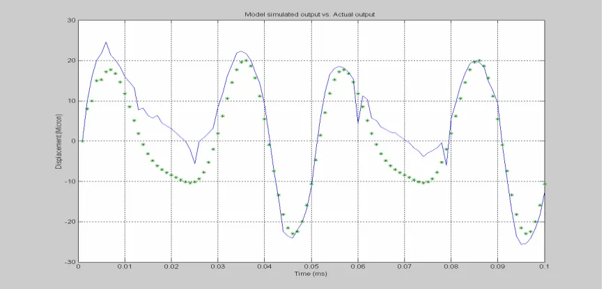
Y (n)= 2.88980 * X (n) + 6.156454 * X (n-4) (3.8)
Figure 3.2 demonstrates simulated output using the time delay model and the actual output from the experiment. Figure 3.3 uses a different input signal, which also consists of two different sinusoid waves in the Figure 3.2. The modeling results are very similar in Figure 3.2 and Figure 3.3.
Figure 3.2: Model simulated output vs. Actual output
series 1(-) – output series 2 (*)– model simulated output value
Y(n)= 2.88980*X(n) +6.156454 *X(n-4)
Figure 3.3: Model simulated output vs. Actual output series 1(-) – output; series 2 (*)– model simulated output value
Y(n)= 2.86289*X(n) +6.23818 *X(n-4)
X(t) = 2V*Sin(2*PI*40*t)+1V*Sin(2*PI*60*t+ ½*PI)
3.4 Second Order Dynamic Model
For control purposes, this time delay model will use as many as four steps of
previously stored values to predict the current output. This will increase the difficulty of
implementing the controller since real-time control is required to achieve high precision.
And, it may cause instability in some situations. So, this time delay model is not practical
for real-time control.
Considering that the magnetostrictive actuation system is a very nonlinear plant, a
higher order dynamic model is necessary to describe its behavior. Using SAS System V8,
a second order dynamic model is obtained. The ARIMA or ARMA is the auto regression
innovations), and current and past values of other time series. The program code is
showed below:
SAS System V8 Program Code:
proc arima data=work.raw;
/*--- Look at the input process ---*/
identify var=x nlag=10;
run;
/*--- Fit a model for the input ---*/
estimate p=3;
run;
/*--- Crosscorrelation of prewhitened series ---*/
identify var=output crosscorr=(input) nlag=10;
run;
/*--- Fit transfer function - look at residuals ---*/
estimate input=( 3$ (1,2)/(1,2) x ) plot;
run;
/*--- Estimate full model ---*/
estimate p=1 input=( 3$ (1)/(1,2) x );
run;
quit;
The values of the numerator and the denominator are then obtained from SAS System
program, when the driving signal is sine wave with frequency of 50Hz and amplitude of 3
volts :
num = [1 -1.2872 0.29768];
den = [7.56088 -7.5816 0.2708];
intercept = 0.901033
Rewriting the dynamic model using State Space Representation:
Du CX Y Bu AX X + = + = &
where matrices A, B, C and D are:
[
2.1628 1.9827]
7.56150 1 2977 . 0 2972 . 1 = − = = − = D C A 0 1 B
respectively. Then eigenvalues λ of matrix A is being checked.
λ > 0
So, this plant is unstable. Then the controllability and observability of the A matrix are
checked. The result indicates it is controllable and observable.
Rearranging the matrix form into differential equations, the plant becomes:
0 0.01 0.02 0.03 0.04 0.05 0.06 0.07 0.08 0.09 0.1 -40
-30 -20 -10 0 10 20 30 40
Tim e(second)
Figure 3.4: Model Simulated Output (dashed line) vs. Actual Output (bold line)
X axis – time (sec); Y axis – displacement (micron) Reference input: Sine wave; Amplitude: 3V; Frequency: 50Hz
Figure 3.4 shows the comparison between the model simulated output and the actual measured output. The model simulated output matches the actual output very well. The
tracking error is acceptable if it is compared with the amplitude of the output signal.
Therefore, this second order dynamic model is more accurate from the simulation results.
This model will be applied in the controller design and experiments implementation in
Reference:
1. R. Venkataraman, P.S Krishnaprasad, “A Model for a Thin Magnetostrictive
Actuator,” Technical Research Report, University of Maryland, College Park, 1998.
2. R. Venkataraman, P.S Krishnaprasad, “Characterization of an ETREMA MP 50/6
Magnetostrictive Actuator,” Technical Research Report, University of Maryland, College
Park, 1998.
3. A.Adly, I. Mayergoyz and A. Bergqvist, “Preisach modeling of magnetostrictive
hysteresis,” Journal of Applied Physics, 69(8), pp.5777-79, 1991.
4. J. B. Restorff, H.T. Savage, A.E. Clark and M. Wunfogle, “Preisach modeling of
hysteresis in Terfonol,” J. Appl. Phys., 67(9), pp 5016-18, 1996.
5. D. Jiles and D. Atherton, “Ferromagnetic hysteresis," IEEE Transactions on
Magnetics, vol. MAG-19, pp. 2183{2185, September 1983.
6. D. Jiles and D. Atherton, “Theory of ferromagnetic hysteresis," Journal of Magnetism
and Magnetic Materials, vol. 61, pp. 48, 1986.
7. V. Basso and G. Bertotti, “Hysteresis models for the description of domain wall
motion,” IEEE Trans. Magn. 32(5), pp.4210-12, 1996.
8. Ralph C. Smith, “A Nonlinear Optimal Control Method for A Magnetostrictive
Actuators, Journal of Intelligent Material System and Structures,” Vol.9, pp. 468-486,
June 1998.
9. Gutierrez, H. M. and Ro, P. I., "Sliding-mode control of a nonlinear-input system:
10. J.-J. E. Slotine and W. Li, “Applied Nonlinear Control,” Prentice Hall, 1991.
11. SAS/ETS Software: “Applications Guide 1,” SAS Institute, 1985.
12. SAS/ETS V8 User's GUIDE: “PROC ARIMA CHAPTER,” SAS Institute, 1985.
13. W. Gao and J.C. Hung, “Variable Structure Control of Nonlinear System: A New
Chapter IV
Controller Design for the Magnetostrictive
Actuation System
4.1 Introduction
As depicted in Chapter I, the alloy Terfenol-D inherently owns some exceptional
magnetomechanical properties and provides a great potential for a variety of transducer
and actuator applications. That potential is now being implemented with the development
of linear and rotary actuators. However, such devices usually require advanced
instrumentation to implement servo-controlled loops, for example, in the case of linear
micropositioning and active vibration control [1]. The performance of a magnetostrictive
actuator is very nonlinear at modest or high drive level and its open loop actuation
performance is not satisfactory if high precision is the interest [2]. Therefore, it’s
necessary to develop a proper controller to reduce the tracking error and obtain better
close-loop actuation performance. In Chapter III, a time-delay model and a second order
dynamic model have been established. These two models will be applied in the
close-loop control.
Krishnaprassad is a bulk and low dimensional model [6]. This model accounts for
magnetic hysteresis, eddy current effects, magneto-elastic effects, inertial effects, and
mechanical damping. From the viewpoint of control, nonlinear model-based control and
optimal control methods have been tried [2, 7]. R D Greenough gave a variable structure
control approach for the magnetostrictive actuator system [8]. J. M. Nealis and R. C.
Smith developed a model reference adaptive control (MARC) for magnetostrictive
transducers operating at fixed, high frequency condition [15, 20]. Due to the existence of
the nonlinearities and saturations in the magnetostrictive actuator, the experimental
results from these approaches are not very satisfactory so far. In this project, a new
modeling method and control approach will be proposed and verified through
experiments.
Figure 4.1 shows the block diagram for implementing close-loop control. The
optical sensor incorporated with the Angstrom Resolver will observe the actuation
displacement driven by the voltage signal from the PWM signal amplifier. Then the
signal from the Angstrom Resolver is directed to the data acquisition board (DSP board),
which communicates with the computer. The DSP board will convert the analog signal
into the digital value used by the computer. The computer then generates a digital control
command obtained from the control algorithm to the D/A part of the DSP board. This
command will be output to the PWM amplifier in analog form, i.e. in voltage. Thus, all
the components in Figure 4.1 form a close-loop control system for the magnetostrictive
Sensor Probe
Tool
Magnetostrictive
Actuator
Compute PID /Sliding Mode
Controller
PWM Signal Amplifier Digital
Computer
DT2823 A/D & D/A DSP Board
Optical Sensor (Angstrom Resolver)
Figure 4.1 Close-loop Control Experiment Block Diagram
In order to simplify the modeling and control problem, 50Hz is chosen as the
working frequency for the actuator since the actuator shows quasi-linear property at this
frequency and 50Hz is often used in applications such as machining.
4.2 PID Controller Design
PID is a classic control algorithm in industry. PID control, namely, proportional,
integral and derivative control, is a traditional and effective close-loop controller for
many mechanical and electrical systems. The main advantage of PID control is that it can
magnetostrictive actuation system is neither perfectly known nor accurate, the PID
controller is tested first to obtain close-loop performance without having an accurate
model.
PID control is an error driven control approach. The ideal PID controller written in
the continuous time domain form is:
0 0 ) ( ) ( ) ( u dt t de Kd dt t e Ki Kp t
u = +
∫
t + + (4.1)Where Kp, Ki and Kd are the proportional, integral, and derivative control gain,
respectively, e(t) is the error, defined as the difference between the desired displacement
and the measured displacement at a specific time t, and u0 is the initial value of the
control input. With u(t) as the current control input. Kp, Ki and Kd can be tuned properly
to get optimized close-loop performance. Table 4.1 illustrates the correlation among
parameters Ki, Kp and Kd and the control performance.
Close-loop Response Rise Time Overshoot Setting Time Steady State Error
Kp Decrease Increase Small Change Decrease
Ki Decrease Increase Increase Eliminate
Kd Small Change Decrease Decrease Small Change
Because Kp, Ki, and Kd are dependent of each other, these correlations may not be
exactly as listed above. In fact, changing one of these variables will change the effect of
the other two. For this reason, Table 4.1 is only a reference when the values of Ki, Kp,
and Kd are determined.
Figure 4.2: Structure of the PID Controller
Figure 4.2 illustrates the structure of this PID controller. In order to implement the
PID controller for the magnetostrictive actuator with a DSP board, it needs to be
discretized. This is to approximate the integral and the derivative terms to the format
suitable for computation by a digital computer. From a numerical point of view, the error
is defined as:
Where e(t) is the error between the value of the desired displacement, Yd and the
displacement value measure Ym. The output of PID controllers will change in response to
a change in the measured displacement.
Integral control
With integral action, the controller output is proportional to the amount of time the
error is present. Integral action eliminates offset. The response is somewhat oscillatory
and can be stabilized somewhat by adding derivative action.
Integral action gives the controller a large gain at low frequencies that results in
eliminating offset and "beating down" load disturbances. The controller phase starts out
at -90 degrees and increases to near 0 degrees at the break frequency. Derivative action
adds phase lead and is used to compensate for the lag introduced by integral action.
Derivative control
With derivative action, the controller output is proportional to the rate of change of
the measurement or error. The controller output is calculated by the rate of change of the
measurement with time.
Derivative action can compensate for a change in measurement. Thus, derivative
action inhibits more rapid changes of the measurement than proportional action. When a
load or set-point change occurs, the derivative action causes the controller gain to move
in the wrong direction when the measurement gets near the set-point. Hence, derivative