Abstract
DEROCHERS, STEVEN JOSEPH. Numerical Study and Feedback Stabilization of a Linear Hydro-Elasticity Model. (Under the direction of Lorena Bociu.)
Fluid-structure interactions arise in a variety of physical, biological, and engineering
problems. Modeling of this phenomenon is crucial in these applications. This work
inves-tigates a total linearization of a free-boundary nonlinear elasticity - incompressible fluid interaction recently derived in [11, 12]. This linearization uses shape optimization
tech-niques and incorporates the geometry of the problem into the analysis. Mathematically,
this model brings up “new” terms–not present in the classical coupling of Stokes flow and
linear elasticity–in the matching of the normal stresses and the velocities on the interface.
It was demonstrated earlier that this PDE system generates a C0-semigroup; however,
unlike in the standard Stokes-elasticity coupling, the well-posedness result depended on
the fluid’s viscosity and the new boundary terms which (among other things) involve the
curvature of the interface. This work implements a finite element-type numerical scheme
for approximating solutions of the fluid-elasticity dynamics and numerically investigate
the dependence of the discretized model on the terms not present in the classical
Stokes-elasticity coupling.
Furthermore, it is known that the classical Stokes-elasticity coupling can be stabilized
by boundary feedback in the form of dissipative matching on the interface [3]. Similarly,
the total linearization can be stabilized; however, in addition to an analogous boundary
c
Copyright 2017 by Steven Joseph Derochers
Numerical Study and Feedback Stabilization of a Linear Hydro-Elasticity Model
by
Steven Joseph Derochers
A dissertation submitted to the Graduate Faculty of North Carolina State University
in partial fulfillment of the requirements for the Degree of
Doctor of Philosophy
Applied Mathematics
Raleigh, North Carolina
2017
APPROVED BY:
Zhilin Li Jesus Rodriguez
Xiao-Biao Lin Lorena Bociu
Biography
Steven Derochers was raised in Morristown, Tennessee. He earned his bachelors of science
degree in mathematics with an honors concentration from the University of Tennessee
in 2011. Afterward, he attended North Carolina State University where he earned his
Acknowledgements
I would like to thank my advisor Dr. Lorena Bociu, my collaborator Dr. Daniel Toundykov,
as well as my family and friends for all their guidance and support. Without their tireless
Table of Contents
List of Tables . . . vi
List of Figures . . . vii
Chapter 1 Introduction . . . 1
1.1 Goals and Challenges . . . 5
1.2 Notation . . . 8
1.3 Outline . . . 9
Chapter 2 Total Linearization . . . 11
2.1 PDE Model . . . 11
2.1.1 Nonlinear PDE System . . . 11
2.1.2 Perturbed PDE System . . . 15
2.1.3 Total Linearization . . . 17
2.2 Well-Posedness of the Total Linearization . . . 20
2.2.1 Resolving Dependence on the Pressure . . . 23
2.2.2 Define Operator A . . . 25
2.3 Semigroup Generation . . . 31
2.3.1 ω-Dissipativity of A. . . 31
2.3.2 Maximality of A . . . 34
Chapter 3 Numerical Results . . . 48
3.1 Prototype Problem . . . 49
3.2 FEM Framework . . . 51
3.2.1 Theoretical Framework . . . 51
3.2.2 Implementation of FEM . . . 57
3.2.3 Testing the Implementation . . . 59
3.3 Numerical Sensitivity Analysis . . . 63
3.3.1 Epsilon Dependence (Constant Coefficient) . . . 64
3.3.2 Epsilon Dependence (Variable Coefficient) . . . 69
3.3.3 Viscosity and Resolvent Dependence . . . 71
3.4 Summary of Observations from the Numerical Analysis . . . 73
Chapter 4 Feedback Stabilization . . . 76
4.1 Dissipative Model . . . 76
4.2 Exponential Stability . . . 78
4.2.1 Energy Identities . . . 79
4.2.2 Preliminary Inequalities: . . . 83
4.3 Important Lemmas . . . 92
Chapter 5 Conclusions and Future Work . . . 98
Bibliography . . . 101
APPENDIX. . . 107
Appendix A Matlab Codes . . . 108
A.1 main.m . . . 110
A.2 AdjustFluidBdry.m . . . 125
A.3 alambdaEx.m . . . 128
A.4 buildsystem.m . . . 135
A.5 calcExtenProb.m . . . 147
A.6 calcExtenStiff.m . . . 154
A.7 calcUbarExt.m . . . 164
A.8 calcVUvec.m . . . 168
A.9 DiffPhi.m . . . 173
A.10 DxKinvMap.m . . . 175
A.11 errorExp.m . . . 175
A.12 Eta.m . . . 176
A.13 getGlobalNodeNum.m . . . 177
A.14 getLocalPhi.m . . . 182
A.15 getMapInfo.m . . . 182
A.16 getMesh.m . . . 185
A.17 getTangVec.m . . . 195
A.18 GEx.m . . . 198
A.19 lamDw.m . . . 206
A.20 load gmsh2.m . . . 207
A.21 Phi.m . . . 217
A.22 quadLine.m . . . 219
A.23 quadTri.m . . . 220
A.24 solidfluid.msh . . . 228
A.25 SolveEigenfunction.m . . . 231
A.26 U1.m . . . 241
A.27 V1.m . . . 242
A.28 w1.m . . . 243
A.29 wplain.m . . . 244
A.30 xKinvMap.m . . . 245
A.31 xKJac.m . . . 245
List of Tables
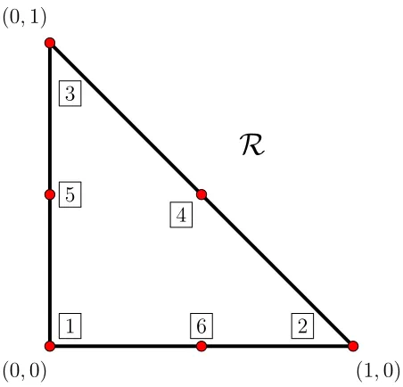
Table 3.1 Quadratic Local Basis Functions over R . . . 55
Table 3.2 Linear Local Basis Functions over R . . . 56
Table 3.3 Eigenvalue Consistency Check Errors . . . 60
Table 3.4 Analytic Solution I Errors . . . 61
List of Figures
Figure 2.1 A sample two-dimensional geometry for a fluid-structure interac-tion problem in steady regime . . . 12
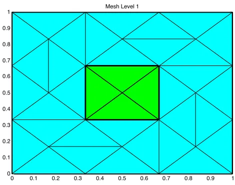
Figure 3.1 “First-level” mesh. Higher level meshes are obtained recursively by connecting the midpoints of the edges for each triangular element with line segments. . . 54 Figure 3.2 Reference TriangleR with labeled local nodes 1 through 6 . . . 55 Figure 3.3 Error exponent in the mesh parameter for Analytic Solution I . . 62 Figure 3.4 Sensitivity w.r.t. parameter ε1 with λ= 1, Mesh Level 2. . . 66
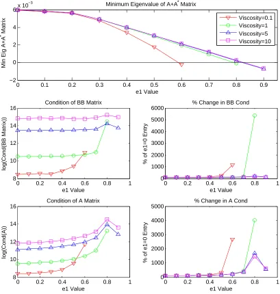
Figure 3.5 Sensitivity w.r.t. parameter ε2 using (3.11) for B(V), with λ = 1,
Mesh Level 2. . . 67 Figure 3.6 Sensitivity w.r.t. parameter ε3, with λ= 1, Mesh Level 2. . . 68
Figure 3.7 Sensitivity w.r.t. parameter ε2 using (3.12) for B(V), with λ = 1,
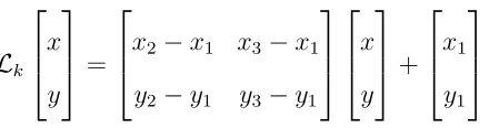
Mesh Level 2. . . 70 Figure 3.8 Minimum eigenvalue of A+A∗ w.r.t. ε1 and viscosity, with λ= 1,
mesh level 1 . . . 72 Figure 3.9 Minimum Eigenvalue of A+A∗ w.r.t. ε1 and λ, with viscosity= 1,
Chapter 1
Introduction
In fluid-elasticity interaction problems, an elastic structure interacts with a gas or fluid
flow. These types of problems have many physical applications, including the flutter of
airplane wings, vibration of turbine and compressor blades, blood flow in arteries, heart
valve dynamics, and interocular dynamics. Fluid-elasticity interactions fall in the category
of free and moving boundary problems. In afree boundary problem, the geometry of the interface surface is typically unknown but remains stationary (not time dependent). In a
moving boundary problem, the common interface is dynamic, and a priori information is provided on the evolution of the geometry. A free and moving boundary value problem
combines the challenges of both of these and requires the unknown boundary to be
determined as a function of time and space. The quintessential example is an elastic
body deforming and moving inside a flowing fluid.
Mathematically, this interaction is described by a partial differential equation (PDE)
system that couples the parabolic (fluid) and hyperbolic (elasticity) phases, where the
key issue is that the traces of the elastic component at the energy level are not defined
nonlinear nature (the equations are nonlinear, and the common boundary is one of the
unknowns in the system and has to be determined as part of the solution), fluid-elasticity
problems continue to be one of the most challenging topics to date. Obviously, the model
has attracted a lot of attention, and its mathematical solvability [6, 13, 18, 19, 22, 21,
25, 33, 34, 35, 36, 39, 41, 53, 58, 55], as well as numerical approximations [23, 28, 40, 57,
56, 48, 50] have been intensively studied in the last three decades.
Various useful simplifications of this models have been considered. A significant
amount of fluid-elasticity interactions fall in the category of small but rapid oscillations
of the solid body, so that the common interface may be assumed static. Another valid
simplification is to consider linearized models, which in some cases provide good
approx-imations of the original nonlinear dynamics. To our knowledge, the first such system
appeared in print as early as 1965 in [16] and was prompted by biomedical applications.
The dynamics was linearized at rest, which effectively amounted to a fixed/cylindrical
ge-ometry on which Stokes flow and linear isotropic elasticity systems were coupled through
suitable stress and velocity matching conditions on the common boundary.
In this thesis, we consider a new, more general linear model for hydro-elasticity,
which was recently proposed in [11, 12]. This work is motivated by the fact that both
stability and control problems related to hydro-elasticity involve the investigation of
this new linearized model. The associated well-posedness analysis for the linear system
is paramount for both stability investigations and optimal control problems subject to
fluid-elasticity interaction, as it is described below:
(i) Optimal Control: The work in [11, 12] was performed in the context of an optimal control problem associated with a free and moving boundary interaction (for
of finding necessary optimality conditions, which provide a characterization of optimal
control, much needed in numerical computations. In this setting, the nonlinear equations
of fluid and solid dynamics (represented by the Navier-Stokes and nonlinear elasticity)
were linearized simultaneously with the free and moving interface between them, using
shape optimization and tangential calculus techniques. This refinement, which we will
address as a ‘total linearization’, led to a markedly different and more complex model,
which agrees with the classical one when the steady regime is the zero equilibrium. In
this new linearization, the matching conditions on the common interface account for
the geometry of the problem through the presence of boundary curvatures. The
well-posedness of the new linearized system is necessary in the investigation of existence and
characterization of optimal control.
(ii) Stability: An important design aspect in many industrial systems and in under-standing many biological phenomena is represented by the stability of equilibrium states
in hydro-elasticity [17, 26, 27, 30]. Essentially, one is interested in whether or not resulting
perturbations grow or decay when an equilibrium is slightly disturbed. The strategy is
to obtain a linearized problem describing the perturbations at first-order, then study the
spectral problem associated with this linearization [31]. For fluid-elasticity interactions,
complexity arises in particular from large structural displacements and the fact that the
position of the common (deformed) interface is not known in advance. This challenge
has been solved by transporting the coupled equations to a fixed reference configuration
[23, 37, 40, 44, 45] or by using transpiration techniques [38, 46, 47, 51, 24, 26, 27, 28]
which are based on modifications of the interface boundary condition. As mentioned
above, the authors in [12] investigated a coupled fluid-structure interaction of an
in-compressible Newtonian fluid and the equations of elastodynamics, subject to small-size
the authors used shape optimization techniques which incorporate the geometry of the
problem in the analysis by linearizing the dynamics equations and the moving boundary
concomitantly. This ‘total linearization’ yields new terms (involving the curvature and
the velocity of the interface) in the matching of normal stresses and velocities on the
in-terface that do not appear in the classical linear Stokes flow and linear elasticity coupling.
The well-posedness analysis for the new linearization [12] was addressed in [9]. The
“new” first-order terms (2.7) present in the Neumann boundary condition for the elastic
solid result in an oblique derivative problem. The hyperbolic component of the
dynam-ics loses regularity under an oblique-derivative condition, even when the coefficients of
those first-order terms are relatively very small. This phenomenon has been well-known
even in scalar hyperbolic equations [42, 14, 52]. Hence the additional terms appearing in
the linearization cannot be trivially handled as mere perturbations of the elastic
com-ponent even if we impose a size condition on them; with the smallness assumption in
place the regularity issues still have to be addressed. In [9] the well-posedness of this
model is investigated via semigroup theory in the special case when the linearization
is performed near a sufficiently smooth low-velocity steady-state regime. In order to ac-commodate the new terms present on the common interface (in both the velocity and
normal stress tensors matchings), the authors (i) derived the basic elliptic theory for the
associated elastic boundary value problem, (ii) constructed a suitable equivalent inner
product on the fluid-structure state space that accommodated not only the specifics of
the hyperbolic component, but also the new perturbed velocity matching condition on
the interface, (iii) identified appropriate conditions that preserved the smoothness of the
advan-perturbation of the evolution operator. The maximality result for the evolution
gener-ator was demonstrated using a variational approach and the Babuˇska-Brezzi theorem
following the strategy in [2]. This argument also provides a convenient framework for a
numerical study of this system via the finite element method. The Babuˇska-Brezzi
ap-proach eliminates the need for divergence-free fluid basis functions in FEM. Moreover,
once the algorithm to solve the maximality system is in place, one can use it to solve the
dynamical problem with prescribed Cauchy data by using the classical formula for the
flow exponential ([49, Thm. 8.3, p. 33]) and corresponding implicit schemes.
One of the traits of the linear semigroup flow approach is that the solution lives in
the associated “finite-energy” state space associated in this case to elastodynamics and
Stokes flow. This regularity is much weaker than employed in the study of fully nonlinear
models. For example, [19] takes advantage of five additional orders of differentiability
in the elastic displacement initial data (total of H6) on top of the finite energy H1 of solutions to isotropic elasticity. Of course, the gain partly follows from the assertion that
linearization is performed around a smooth solution to the nonlinear problem in the first place, such as linearization near equilibrium. The analysis in [9], however, shows that if the
linearization takes into account geometry of the domain and is performed near a nonzero
steady regime then existence of finite-energy solutions likely requires a sufficiently large
viscosity—this aspect was irrelevant in the simple classical Stokes-elasticity coupling. The
analytic study in [9] does not not provide precise quantitative estimates on the relative
parameter sizes, and the current paper aims at investigating this aspect further.
1.1
Goals and Challenges
effect of the new, when compared to the classical model, trace terms on the discretization.
In particular, we numerically examine:
1. how the ellipticity constants and matrix condition numbers in the associated
dis-cretized system are affected by the magnitude of the boundary terms present in
the matchings of the normal stress tensors and of the velocities on the common
boundary (see (2.7)–(2.8) below).
2. whether the size of the boundary terms may affect the convergence rates in the
numerical scheme.
The structure of the interface conditions ((2.7) and (2.8) below) is quite involved and
the coefficients depend on the exact solution to the associated steady-regime problem
around which the linearization is performed. A direct investigation would thus require
an exact solution to a nonlinear hydro-elastic system. In addition, elements with curved
boundaries would be needed to consider the curvature terms. We can partly
circum-vent these difficulties by noting that the semigroup-wellposedness analysis [9] critically
depends only on the following properties of the linearized system:
(i) The norms (in appropriate spaces) of the fluid velocity, the pressure, and of the
deformation in the steady regime around which the linearization is performed, and
the size of the fluid viscosity relative to these norms.
(ii) The fact that the additional terms (when compared to classical coupling of Stokes
and linear elastodynamics) on the interface can be decomposed into zero-order and
first-order tangential derivatives only, without normal components.
geom-Based on these observations, we consider a modified system which admits simplified
interface conditions and piecewise-flat geometry. At the same time, this model partly
recreates the original dynamics by incorporating zero and first-order perturbations on
the interface. Thus a large-curvature scenario is simulated by directly adjusting the size
of the coefficients of certain trace terms.
The system is numerically implemented using a finite element scheme with
Taylor-Hood elements and illustrates optimal convergence rates [7] for the considered analytic
test-solutions. The dependence of the numerical system on the size of the parameters
specific to this model is then investigated.
II. Secondly, we investigate how the new linear model in [9] compares to classical linear coupling of fluid and elasticity with respect to stabilization properties. The
cou-pling between linear elasticity and the Stokes system has been investigated in a recent
series of papers by Avalos and Triggiani (in [1] the authors studied spectral properties of
the semigroup generator; [2], by Avalos and Dvorak, provides an alternative proof of the
maximality argument; [4] addresses semigroup well-posedness of a damped model; and [5]
treats the backward uniqueness problem). The least amount of damping required for
sta-bilization of the Stokes-elasticity model is the boundary interface feedback. The uniform
exponential stability was demonstrated in [3]. Such a feedback represents a refinement
accounting for the slip condition on the interface that dissipates energy through friction
[54, p. 240]. From an operator theory viewpoint, the corresponding boundary term shifts
the generator spectrum to the left, away from the imaginary axis. In comparison, we
work with the model obtained in [9] and we demonstrate that a “suitably damped”
fluid-structure interaction model, linearized around a steady regime is exponentially stable.
Unlike the Stokes-elasticity scenario, the stability in this case is contingent on the
[41]. Moreover, the dissipation through the interface naturally competes with the energy
of the steady regime, hence the stability property may be lost if the steady regime’s
energy is too high. This interplay of forces leads to interesting correlations between the
stability of the system and the relative values of the physical parameters as presented in
the discussion below.
1.2
Notation
The following notation, following the conventions used in [8], will be used throughout
this work.
• Mm×n denotes the real m×n matrices, and
Mm =Mm×m.
• A∗ denotes the (conjugate) transpose of the matrix A.
• A..B = Tr(A∗ ·B) ∈ R is the Frobenius product in M2 or
M3 depending on the
size of the matrices A and B.
• (Df(a))ij = ∂jfi(a) ∈ M3 is the Jacobi matrix at a ∈ X of any vector field
f = (fi) :X ⊂R3 →R3.
• IfT is a 2-tensor, then DT is a 3-tensor whose contraction with a vector gives
[(DT)e]ij = (∂kTij)ek.
For a given vector n,
∂T
• DivT(a) =∂jTijei ∈R3 is the divergence of any 2nd-order tensor field T = (Tij) :
X ⊂R3 →
M3 ata∈X.
• dΩ(x) =
infy∈Ω|y−x| Ω6=∅
∞ Ω =∅
is the distance function from a point xto the set
Ω⊂Rk.
• bΩ(x) = dΩ(x)−dΩc(x), for x ∈ Rk is the oriented distance function from x to
domain Ω ⊂ Rk. Thus ∆b
Ω = Tr(D2bΩ) is the additive curvature of Γ = ∂Ω, and
D2b
Ω is the matrix of curvatures of Γ.
Also note the following bilinear forms, norms and duality pairings:
• The bilinear form (·,·)X indicates the inner product on a given Hilbert space X.
• Product spaces [X]kare abbreviated with boldX. Likewise the dual [X0]k ∼= ([X]k)0 will be denotedX0. The value of k will be clear from the context.
• k · kX will denote the norm on X.
• For a Lipschitz compact boundary-less manifoldM, let{·,·}1
2,M denote the duality
pairing between the Sobolev spaces H−1/2(M) and H1/2(M).
1.3
Outline
The remainder of this work proceeds as follows:
• Chapter 2 introduces the total linearization obtained by the authors in [12]. It will also highlight the important aspects of the well-posedness argument for this
• Chapter 3 introduces a prototype system as a substitute for the original total linearization. It then constructs and tests a finite element method on this prototype
problem. Finally, it investigates the sensitivity of parameters in the system with
respect to well-posedness.
• Chapter 4 shows the feedback stability of the total linearization and contrasts with the argument found in [3].
• Chapter 5 provides a summary of the observations found in the preceeding chapters as well as avenues for future work.
Chapter 2
Total Linearization
In order to understand the numerical sensitivity analysis in Chapter 3, it is important to
understand the contrast between the classical Stokes-linear elasticity system and the total
linearization found in [12] as well as the underlying well-posedness argument developed
in [9] for this new linearization. The well-posedness argument adapts the argument found
in [2] to the new challenges presented by the total linearization.
2.1
PDE Model
2.1.1
Nonlinear PDE System
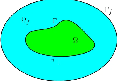
Let D ⊂ R3 be an open, bounded, and compact domain with fixed boundary δD =
Γf. D contains an elastic solid with domain Ω which is surrounded by a fluid domain
Ωf ⊂ D. The union of these non-overlapping subdomains is the full domain D = Ω∪
Ωf. Furthermore, the interface between Ω and Ωf is given by Γ = δΩ. A sample
Ω
Ω
f
n
Γ
Γ
f
Figure 2.1: A sample two-dimensional geometry for a fluid-structure interaction problem in steady regime
This work assumes that the fluid under consideration is viscous, Newtonian,
homoge-nous, and incompressible. Furthermore, the fluid satisfies the no-slip conditions on the
steady state case, the PDE model is given by
−ν∆w + Dw·w + ∇p = v
Ωf
on Ωf
div w= 0 on Ωf
w= 0 on Γf
−DivT =v
Ω on Ω
Tn=σ(p, w)n on Γ
ϕ=IΓf on Γf.
(2.1)
And the non-steady state system is given by
wt−ν∆w + Dw·w + ∇p = v
Ωf(t)
on Ωf(t)
div w= 0 on Ωf(t)
w= 0 on Γf
ϕtt◦ϕ−1−[J(ϕ)◦ϕ−1] DivT =v
Ω(t) on Ω(t)
w◦ϕ=ϕt on Γ(t)
T ·n =σ(p, w)n on Γ(t)
ϕ=IΓf on Γf.
(2.2)
In systems (2.1) and (2.2), we have the following:
• The fluid dynamics satisfy the Navier-Stokes equations with no-slip conditions on the outer boundary Γf. The viscosity of the fluid is ν > 0, and the fluid strain
Dw is the matrix of partial derivatives for the fluid velocity w.
• The domain of the elastic solid Ω, referred to henceforth as the solid domain, is char-acterized according to a mappingϕacting in a fixed reference domain (Lagrangian formulation). The evolution of the fluid domain Ωf is seen via the structural
defor-mation through the boundary interface Γ. LetΩe ⊂ D be a reference configuration
for the solid domain. Further, let eΓ =∂Ω be its boundary. Thene Ωef = D \Ω cane
be taken as the reference configuration for the fluid domain (again, with Γ as thee
boundary interface between the two domains). The full domain D can be charac-terized by a smooth, injective, orientation-preserving map ϕ: D → D, x 7→ ϕ(x). If x ∈ Ω,e ϕ(x) represents the position of the material point x. In the case where
x ∈ Ωef, ϕ(x) is defined to be an arbitrary extension of the restriction of ϕ|
e
Γ that
preserves the bounary Γf. That is to say, ϕ= Id on Γf. Define J(ϕ) = det(Dϕ) to
be the Jacobian of the deformation mappingϕ. The orientation-preserving property of ϕgives us that J(ϕ)>0.
• The fluid is coupled with the St. Venant-Kirchhoff equations which model large displacement/small deformation elasticity. The equations of elasticity are writen
on the deformed configuration Ω using the Cauchy stress tensor T:
T = [J(ϕ)−1P ·(Dϕ)∗]◦ϕ−1.
The Cauchy stress tensor is given in terms of the Green-St. Venant nonlinear strain
tensor σ(ϕ) and the Piola transformP, given by
P =Dϕ[λeTr(σ(ϕ))I + 2µeσ(ϕ)] and σ(ϕ) =
1 2[(Dϕ)
∗
where λe and µe are the Lam´e parameters of the material. Here the “e” subscripts
refer to the elasticity and are used to differentiate the Lam´e parameters from the
resolvant value λ used later in this work. This leads to the matching of the normal stress tensors Tn and σf(p, w)n on the interface Γ using
σf(p, w) = 2νε(w)−pI ,
where n is the unit outward normal vector with respect to Ω.
For the steady regime (2.1), well-posedness analysis appears in [33] and [60]. Similarly,
well-posedness in the non-steady regime case (2.2) can be found in [19]. Because of this,
we assume that the nonlinear systems are well-posed and possess sufficient regularity to
take advantage of the existence result from [9], discussed below, for the total linearization.
2.1.2
Perturbed PDE System
The next step in deriving the total linearization is to perturb the nonlinear system (2.2).
This is done in the forcing termv on the right hand side of the system. The forcing term v is replaced by the perturbationvs(x, t) which depends linearly on parameter s∈[0, s0]
for some small s0 given v0(x, t).
vs(x, t) = v(x) +sv0(x, t)
This type of perturbation arises in optimal control problems, and the case when the state
of the entire hydro-elastic system is controlled from the fluid domain or its outer layer is
of particular interest.
Ωf and Ω change as the time parameter t changes. The functions (ϕs, ws, ps) solve the
perturbed system (2.3).
∂ws
∂t −ν∆ws+ Dws·ws + ∇ps = vs
Ωs f(t)
Ωs f(t)
divws= 0 Ωsf(t)
∂2 ∂t2ϕs
◦ϕ−s1 −[Js(t)◦ϕ−s1] DivTs =vs
Ωs(t) Ω
s(t) = ϕ
s(t)(Ω)e
ws=
∂
∂tϕs◦ϕ
−1
s Γs(t) = ϕs(t)(eΓ)
Ts·ns(t) = (2νε(ws)−psI)ns(t) Γs(t)
ws= 0 Γf
ϕs(·,0) =ϕ0,
∂ϕs
∂t (·,0) =ϕ
1, w
s(·,0) =w0, ps(·,0) =p0
(2.3)
where ns(t) is the unit normal exterior to the solid domain Ωs(t). As before, Js(t) is the
Jacobian of the deformation ϕs(t). Ts and Ps are given by
Ts = [(1/J(ϕs))Ps·(Dϕ)∗]◦ϕ−s1
Ps = Dϕs[λeTr(σe(ϕs))I+ 2µeσe(ϕs)].
The strategy here is to differentiate system (2.3) with respect to parameter s at s = 0 about a solution (w, p, ϕ) to the steady regime system (2.1) using shape calculus techniques. The resulting linearized system for the unknown s-derivatives of ws, ps, and
2.1.3
Total Linearization
In order to fully describe the total linearization, a bit more notation is required. Below,
the prime “ 0 ” notation is used to indicate derivatives in the s parameter evaluated at s= 0, i.e.,
ϕ0 = ∂ ∂sϕs(t)
s=0
, w0 = ∂ ∂sws(t)
s=0
, and p0 = ∂ ∂sps(t)
s=0
.
Next, define the elastic displacement vector (for linearized elasticity on the deformed
configuration) as
U0 =ϕ0◦ϕ−1.
Then, let
Θ =Dϕ◦ϕ−1 = [D(ϕ−1)]−1. (2.4)
Thus,Dϕ0◦ϕ−1 = (DU0)Θ. The nonlinear strain tensor associated with ϕis given by
σ(ϕ)◦ϕ−1 = 1 2[Θ
∗
Θ−I],
and the linearized strain associated with U0 can then be written as
σ0(ϕ)◦ϕ−1 = 1 2[Θ
∗
(DU0)∗Θ + Θ∗(DU0)Θ]
= 1 2[Θ
∗
(DU0)Θ + (Θ∗(DU0)Θ)∗].
If we let DU0 = Θ∗(DU0)Θ, then we can write the strain as the symmetrized gradient
conjugated by Θ.
E(U0) = σ0(ϕ)◦ϕ−1 = 1 2[DU
0+ (DU0)∗
Then, since Tr(σ0(ϕ)◦ϕ−1) = Tr(Θ∗(DU0)Θ), we have
Σ(σ0(ϕ)◦ϕ−1) = λeTr(σ0(ϕ)◦ϕ−1)I+ 2µe(σ0(ϕ)◦ϕ−1)
= λeTr(DU0)I +µe[DU0+ (DU0)∗]
= Σ(E(U0)).
Note the similarity to the Piola transform P above. Furthermore, define
e
Σ(V) = ΘΣ(E(V))Θ∗.
Then the Cauchy stress tensor T is given by
T =
1
det(Dϕ)Dϕ·Σ(σ(ϕ))·(Dϕ)
∗
◦ϕ−1
= 1
det(Θ)Θ·Σ
1 2[Θ
∗Θ−I]
Θ∗.
This, as calculated in [12], leads to the linearized Cauchy stress tensorT0, given by
T0 = 1 det ΘΣ(e U
0
) + (DU0)T . (2.6)
With this, we are prepared to state the existence theorem of the total linearization
found in [9].
Theorem 2.1.1 (The total linearization around a steady regime [9]). Assume that for all s ∈[0, s0], (2.3) is well-posed on [0, T] such that for >0 and all t ∈[0, T], we have
ws(t)∈W
11
4+,4(Ωef(t)),p(t)∈W 7
4+,4(Ωef(t))andϕ(t)is aW 15
4+,4(D)diffeomorphism.
(ϕ0, w0, p0) associated with (2.3) solves the steady regime problem (2.1). Then (ϕ0, w0, p0)
satisfy the following cylindrical (i.e. on a time-independent space domain) evolution problem:
wt0 −ν∆w0 + (Dw0)·w+Dw·w0+ ∇p0 = v0
Ωf in Ωf
divw0 = 0 in Ωf
w0+ (Dw)U0 =Ut0 in Γ
∂2
∂t2U 0−
(det Θ) DivhT0(U0)i =v0
Ω in Ω
T0(U)n= (2νε(w0)−p0I)n+B(U0) on Γ
w0 = 0 on Γf
ϕ0(0) = 0, w0(0) = 0, ϕ0t(0) = 0.
(2.7)
where the boundary operator B is given by
B(V) = (T +pI−2νε(w))·[(DΓV)∗n+ (D2bΩ)VΓ]
−hV, ni−DivΓ(T) +
h
∂p
∂nI−2ν ∂ε(w)
∂n
i
·n +(DT)V ·n+ div(V)T ·n− T ·(DV)∗·n .
(2.8)
Recall from Section 1.2 that the oriented distance function for domain Ω is given by
bΩ. In this case, D2bΩ in B(V) yields information on the curvature of the Γ boundary
interface, bringing the geometry of the problem more deeply into the analysis.
boundary term cannot be dismissed as merely a small perturbation ofU0. The hyperbolic portion of the dynamics may lose regularity even when the first-order coefficients of the
oblique-derivative condition are relatively small. This phenomenon is well-known even in
scalar hyperbolic equations [42, 14, 52].
2.2
Well-Posedness of the Total Linearization
The authors in [9] established the well-posedness of (2.7) using semigroup methods. To
follow their work, equip the space L2(Ω) with the equivalent inner product
(V, W)L2 Θ(Ω) =
Z
Ω
1
det ΘhV, Wi (2.9)
assuming that det(Θ) > 0 is bounded below on Ω. Similarly, for H1(Ω), the space of
elastic displacements, define the equivalent inner product
(V, W)H1(Ω) = (V, W)L2 Θ(Ω)+
Z
Ω
1
det ΘΣ(e V)..DW +
Z
Ω
T0(V)..DW . (2.10)
The functions Ut0 and U0 are elements of these spaces respectively. At this time, we also define the bilinear form aS(V, W) by
aS(V, W) = (V, W)H1(Ω)− {B(V), W}1
2,Γ. (2.11)
Finally, let the fluid velocity space be given by
H1Γ
f(Ωf) =
n
ϕ∈H1(Ωf)
ϕ|Γf = 0
o
This leads to the definition of the state space for the full coupled system,
H =H1(Ω)×L2Θ(Ω)× Hf
where
Hf =
n
V ∈L2(Ωf)
div(V) = 0,hV, ni|Γf = 0
o
.
The authors in [9] equip H with the following bilinear form:
U0 V0 w0 , e U e V e w H
= (U0,Ue)H1(Ω)+
V0−(Dw)U0,Ve −(Dw)Ue
L2 Θ(Ω)
+ (w0,we)L2(Ω
f)
(2.13)
wherewis an extension of the steady “linearization velocity”wto the entire control vol-ume domainD. This bilinear form defines an equivalent inner product onH with assump-tions on the smallness of w and that w is regular enough to admit a small kDwkL∞(D).
We will suppress the underline notation on w when no confusion will arise.
Note that the coefficients in the total linearization (2.7) depend on the steady regime
solution (w, ϕ, p) from system (2.1). As such, some constraints on the size and regularity of (w, ϕ, p) are needed. These assumptions, enforced in [9], are reasonable based on the smoothness of solutions verified in [19].
Assumption 2.2.1. (Sufficient conditions on the Nonlinear Steady Regime [9, Assump-tion 3]) Assume that the funcAssump-tions (ϕ, w, p) satisfying the steady regime problem (2.1) obey the following conditions:
(i) w has an extension to D:
w∈C1(D) and w=w in Ωf
(ii) The coefficients of first-order terms in V in B(V) defined in (2.8) must be multipliers for H1/2(Γ) topology. Specifically,
Tjk, p, and , δxiwk
are multipliers on H1/2Γ. The coefficients of zero-order terms in V must be in
L∞(Γ), i.e.
δxiTjk, δxip, and δxiδxjwk belong to L
∞
(Γ)
Since H1/2(Γ) dim,→=2 L4(Γ), then by [59, Prop. 1.1, p.105 with s = 1 2, p =
2, q2 = 12, q1 = ∞, and r1 = 4, r2 = 4] to be a multiplier on H1/2(Γ) it
is enough to live in W12,4(Γ)∩L∞(Γ). So conditions (R-2) are stronger. The
spaceL∞(Γ)containsW12+ε,4(Ωor Ωf). (Note that by [59, Prop. 1.1], any space
Wj+34+ε,4(Ω or Ωf), j ∈Z+ forms a Banach algebra). We will therefore assume
that
• w∈W114+ε,4(Ωf)
• p∈W74+ε,4(Ωf)
• ϕ is a W154 +ε,4(Ω) diffeomorphism
(iii) For the boundary, we assume that D2b
Ω ∈ L∞(Γ) and that n is a multiplier
with respect to H1/2(Γ) topology. Since the regularity of b
boundary [20], it suffices to assume that Γ∪Γf is of class C2 (and locally on
one side of the fluid domain).
(b) Smallness:LetRdenote the regularity spaceW154+ε,4(Ω)×W 11
4+ε,4(Ωf)×W 7
4+ε,4(Ωf).
Assume that
r=k(ϕ−Id, w, p)kR
is small enough so that there are constants 0< c=c(r) <1 and ω =ω(r)≥ 0, for which any functions wˆ∈H1(Ωf), Uˆ ∈H1(Ω), and Vˆ ∈L2Θ(Ω) satisfy
(i) {B( ˆw) + (Dw) ˆU ,w}ˆ 1
2,Γ<(c)(2ν)
RT
0
R
Ωf ε( ˆw)..ε( ˆw) +Ck
ˆ Uk2
H1(Ω)
(ii) 2
( ˆV ,(Dw) ˆU)L2Θ(Ω)
≤c
kVˆk2
L2
Θ(Ω)+k(Dw) ˆUk
2+kUˆk2
H1(Ω)
(iii) R
Ω(DVˆT..DVˆ|+
{B( ˆV ,
ˆ V}1
2,Γ
≤c
kVˆk2
L2 Θ(Ω)
+RΩdet(Θ)Σ( ˆe V)..DVˆ
(iv) ( ˆU ,(Dw) ˆU)H1(Ω)−((Dwˆ)w,wˆ)L2(Ω
f)+{B( ˆU),w}ˆ 12,Γ
−(Dw) ˆV ,Vˆ −(Dw) ˆU
L2 Θ(Ω)
−2νR
Ωf ε( ˆw)..ε( ˆw)
≤ωkUˆk2
H1(Ω)+kVˆk2L2 Θ(Ω)
The existence of such c(r) and ω(r) for all small r is justified through Proposition 2.2.2 and Proposition 2.2.1 below.
2.2.1
Resolving Dependence on the Pressure
Typically, the first step in analyzing well-posedness of systems like (2.7) is to resolve the
dependence of the dynamics on the pressure p0. The usual Leray projection cannot be applied due to the interface coupling, since the Leray projection requires that the fluid
problem.
−∆p0 = (Dw0)∗..Dw in Ωf
p0 = h2νε(w0)n, ni+hB(U0), ni − hT0(U0)n, ni on Γ
δnp0 = hν∆w0, ni on Γf
The solution p0 is found using the following harmonic extension maps.
p0 =π0(U0, w0) = De(h2νε(w0)n, ni+hB(U0), ni − hT 0
(U0)n, ni)
+Nf(hν∆w0, ni) +A−1((Dw0)∗..Dw)
where A = −∆, D(A) = {f ∈ H1(
e
Ωf)|Af ∈ L2(Ωef) and f|Γf = 0 = δνf|Γf}, and the
Dirichlet extension De :H−1/2(eΓ)→L2(Ωef) and Neumann extensionNe :H−3/2(Γf)→
L2(
e
Ωf) are given by
h=De(g) ⇔
∆h = 0 in Ωf
h = g on Γ ∂h
∂n = 0 on Γf
h=Nf(g) ⇔
∆h = 0 in Ωf
h = 0 on Γ ∂h
2.2.2
Define Operator
A
After the dependence on the pressure is resolved, it is possible to rewrite system (2.7) as
an evolution problem:
d dty
0
=Ay0 (2.14)
on the state space H where y0 =
U0 V0 w0
∗
. The operator A is given by
A: U0 V0 w0
∈ D(A)⊂H →
V0 −S(U0)
ν∆w0−(Dw0)·w− ∇π0(w0, U0)
∈H . (2.15)
where the elasticity operator S is defined by
S(V) =−det(Θ) Div[T0(V)] +V (2.16)
In [9], the identity was added to S for convenience to ensure the ellipticity of the asso-ciated operator; however, semigroup well-posedness is not affected by a bounded
pertur-bation. Here the (Dw)·w0 term in the fluid equation was dropped as a small bounded perturbation of w0. Likewise, a U0 term was included in the elastic equation for conve-nience that also has no effect on well-posedness.
If it can be shown that the operator A generates a C0-semigroup, then the total
linearization is well-posed. With initial conditionsy0 =
U0 V0 w0
∗
solution to the total linearization is given by
U0(t) Ut0(t) w0(t)
=etA
U0 V0 w0
The semigroup exponential notation becomes more clear here when we notice the
parallels to an exponential growth or exponential decay differential equation. Section 2.3
outlines the proof justifying the authors’ claim in [9] that Agenerates aC0-semigroup to
complete the well-posedness argument, and the remainder of this section will define the
domain of Aalong with additonal observations made in [9] that are needed in the proofs
of Section 2.3.
The domain D(A) of the generator is a subspace of H2(Ω)×H1(Ω)×H1(Ωf) as seen
in [9, Sec. 6.3, p.1986-1987]. The exact conditions on y0 =
U0 V0 w0
∗
in order to
apply A are given below.
Definition 2.2.1. The domain D(A) of the operator A given by (2.15) is the subset of H2(Ω)×H1(Ω)×H1(Ω
f) with the following restrictions. For all
U0 V0 w0
∗
∈ D(A),
(i) (U0, V0, w0)∈H
(ii) V0 ∈H1(Ω) (Consequently, V0|Γ is defined in L2(Γ), in fact H1/2(Γ).)
(iii) w0 ∈H1(Ω
f) and for some function π0 ∈L2(Ω)
−∆w0+∇π0 ∈L2(Ωf)
(iv) S(U0)∈L2(Ω) in the sense that for any Ψ∈C∞
c (Ω), there is a V ∈L2(Ω) where
(V,Ψ)L2
Θ(Ω) = (U
0
,Ψ)H1(Ω)− {B(U0),Ψ}1 2,Γ
(v) w0 =0 in L2(Γ f).
(vi) w0+ (Dw)U0 =V0 in H1/2(Γ).
(vii) π0 =π(w0, U0) and T 0
(U0)n− B(U0) = [2νε(w0)−π(w0, U0)I]n in H−1/2(Γ).
The following observations from [9] are needed in the proofs given in Section 2.3.
Proposition 2.2.1. ([9, Prop 4.1]) The functional
ˆ w7→
Z
Ωf
ε( ˆw)..ε( ˆw)
!1/2
defines an equivalent norm on the space HΓ1
f(Ωf).
Proposition 2.2.2. (Boundary operator B [9, Prop. 6.2]) The transformation V 7→ B(V) continuously extends from H2(Ω)→L2(Γ) to a bounded linear mapping H1(Ω)→
H−1/2(Γ)
Proposition 2.2.3. (Bilinear FormaS, [9, Prop 6.3]) Consider the linear transformation
H1(Ω)→[H1(Ω)]0:
V 7→ W 7→H2(Ω) for W ∈H1(Ω) If V belongs to
D(S) =nV ∈H2(Ω)
T
0
(V)n− B(V) = 0o then for any W ∈H1(Ω)
aS(V, W) = (S(V), W)L2
Θ(Ω) (2.17)
Moreover, if Assumption 2.2.1 holds, then the bilinear form aS is continuous elliptic
on H1(Ω). By maS and MaS, we will denote respectively the ellipticity constant and the
continuity modulus for aS:
maSkVk
2 ≤a
S(V, V)≤MaSkVk
2
for V ∈H1(Ω).
Proposition 2.2.4. (Extending T0 ·n− B to Functions in H1(Ω), [9, Prop. 6.5]) Let
V ∈ H1(Ω). Assume S(V) ∈ L2(Ω) in the sense that there is F ∈ L2(Ω) such that for
any test function Ψ∈Cc∞(Ω), we have
aS(V,Ψ) = (F,Ψ)L2
Θ(Ω) (2.18)
Suppose Assumption 2.2.1 holds so that aS is H1(Ω) elliptic. Then R=T 0
(V)n− B(V) is uniquely defined as an element of the dual space H−1/2(Γ), and we have the identity
If V ∈ H2(Ω), then the duality pairing {·,·}
1
2,Γ amounts to integration on the boundary
Γ.
Proposition 2.2.5. (HomogeneousS-Dirichlet Problem, [9, Prop 6.7]) LetG∈H−1(Ω),
then for any λ∈R, the homogeneous Dirichlet boundary value problem,
λ2V0+S(V0) = G in Ω
V0 = 0 in Γ
(2.20)
has a unique weak solution V0 ∈H01(Ω) in the sense that
λ2(V0, W)L2
Θ(Ω)+aS(V0, W) = (G, W)H−1(Ω):H01(Ω)
for all W ∈H1
0(Ω) with the bilinear form aS given by (2.11).
Proposition 2.2.6. (S-Dirichlet Problem, [9, Prop. 6.8]) Let F ∈ [H1(Ω)]0 and R ∈
H1/2(Γ). For any λ ∈
R, the boundary value problem
λ2V +S(V) = F in Ω
V = R on Γ
(2.21)
has a unique weak solution V ∈H1(Ω) in the sense that V =V0+Ve where Ve ∈ H1(Ω)
has trace R in H1/2(Γ). And V0 ∈ H01(Ω) is the weak solution to the Dirichlet problem
(2.20) with
for all W ∈H1
0(Ω). Thus by (2.2.5), V0 and Ve satisfy the variational identity
λ2(V
0, W)L2
Θ(Ω)+aS(V0, W)
= (F, W)H−1(Ω):H1
0(Ω)−aS(V , We )−λ
2(
e
V , W)L2 Θ(Ω)
(2.22)
for all W ∈H1
0(Ω). Equivalently,
λ2(V, W)L2
Θ(Ω)+aS(V, W) = (F, W)H−1(Ω):H01(Ω) (2.23)
for all W ∈ H1
0(Ω). Moreover, for the ellipticity and continuity constants maS and MaS
of aS, and any δ >0, there are constants Cp, Ce, Ce,δ (detailed in the proof ) such that
λ2C
pkV0kL2
Θ(Ω)+maSkVkH 1(Ω)
≤ 2kFkH−1(Ω)+λ2CpCe,δkRkHδ(Γ)+MaSCekRkH1/2(Γ)
(2.24)
Definition 2.2.2. (S-Dirichlet Extension, [9, Def. 6.9]) Denote by DS,λ2 the bilinear
solution map DS,λ2 : (F, R)7→V to the Dirichlet problem given by (2.21) in Proposition
2.3
Semigroup Generation
The next step in the well-posedness argument is to show thatAgenerates aC0-semigroup.
Unfortunately, the system
d dt
U0 Ut0 w0
=A
U0 Ut0 w0
(2.25)
does not allow for a direct application of the Lumer-Philips theorem, as was the case in
[2].
Theorem 2.3.1. (Lumer-Phillips [various, e.g. [49, Thm. 4.3, p.14]]) LetG be a linear operator with dense domain D(G) in Banach space X. If G is dissipative and there is a λ0 > 0 such that the range, R(λ0I −G), of λ0I −G is X, then G is the infinitesimal
generator of a C0-semigroup of contractions on X.
Instead, the authors in [9] identified a bounded perturbation of A which is maximal
dissipative, hence Lumer-Phillips can be applied to the perturbation. This is enough to
conclude that A generates a C0-semigroup [49, p.12].
2.3.1
ω
-Dissipativity of
A
In order to apply the Lumer-Phillips theorem 2.3.1 to a bounded perturbation of A,
first dissipativity must be shown, i.e. show ω-dissipativity of A itself. To emphasize the importance of having “large enough” viscosity in the total linearization, we include the
following lemma with proof from [9].
Lemma 2.3.1. (Dissipativity) For viscosity ν > 0, there exists a r0 = r0(ν) > 0 and a
r0 in Assumption 2.2.1 the operator
Aω =A−ω(r)
1 1 0 is dissipative.
Proof. Recall that
A U0 V0 w0 = V0 −S(U0)
ν∆w0−(Dw0)w− ∇π(w0, U0)
.
Define y =
U0 V0 w0
∗
∈ D(A). Since the conditions found in Assumption 2.2.1 hold for all small r, it is enough to show the following inequality.
(Ay, y)H ≤ω(r)kU0k2
H1(Ω)+kV0k2L2 Θ(Ω)
From the inner product on H, we have
(Ay, y)H = (U0, V0)H1(Ω)−(S(U0) + (Dw)V0, V0−(Dw)U0)L2 Θ(Ω)
+ (ν∆w0− ∇π0, w0)−((Dw0)w, w0)L2(Ω
Next apply the definition of aS(·,·) and the identity (2.19).
(Ay, y)H = (U0, V0)H1(Ω)−(U0, V0)H1(Ω)+ (U0,(Dw)U0)H1(Ω)
+{B(U0), V0−(Dw)U0}1
2,Γ+{T
0
(U0)n− B(U0), V0−(Dw)U0}1 2,Γ
−((Dw)V0, V0−(Dw)U0)L2 Θ(Ω)
+(ν∆w0− ∇π, w0) L2(Ω
f)−((Dw
0)w, w0) L2(Ω
f)
(2.26)
Because divw0 = 0 ⇒ Div((Dw0)∗) = 0, we have ν∆w0 = 2νDiv(ε(w0)). Then recalling that n is the unit normal outward with respect to the solid domain
(ν∆w0− ∇π, w0)L2(Ω
f) = (2νDiv(ε(w
0
))− ∇π, w0)L2(Ω
f)
= −2ν
Z
Ωf
ε(w0)..ε(w0)− {(2νε(w0)−πI)n, w0}1 2,Γ.
By the velocity matching condition (vi) and the identification (vii) of 2.2.1, we have
{T0(U0)n− B(U0), V0−(Dw)U0}1
2,Γ ={(2νε(w
0
)−πI)n, w0}1 2,Γ.
Thus we may cancel terms in (2.26). Finally, use the velocity matching condition to
expand
{B(U0), V0−(Dw)U0)1
2,Γ ={B(U
0), w0}
1 2,Γ.
This leaves us with
(Ay, y)H = (U0,(Dw)U0)H1(Ω)−((Dw0)w, w0)L2(Ω
f)
+{B(U0), w0}1
2,Γ−((Dw)V
0
, V0−(Dw)U0)L2 Θ(Ω)
−2ν
Z
Ωf
Because B defines a continuous trace operator on H1(Ω) →H−1/2(Γ) using Proposition
2.2.2, we can estimate
(Ay, y)H ≤ C(r)kw0k2 H1(Ω
f)+ω(r)
kU0k2
H1(Ω)+kV0k2L2 Θ(Ω)
−2ν
Z
Ωf
ε(w0)..ε(w0)
where C(r) and ω(r) can be chosen continuous monotone increasing in r with C(0) = 0 =ω(0). We needr to be small enough to ensure that
C(r)kwkˆ H1(Ω
f) ≤2ν
Z
Ωf
ε( ˆw)..ε( ˆw)
for all ˆw ∈ H1(Ω
f). Such an r always exists by the property of C(r) and Proposition
2.2.1. This is where the viscosity of the fluid plays its role in counteracting the potentially
destabilizing effect of the trace operatorB. In contrast with the classical Stokes-elasticity system where any positive viscosity is sufficient, a “large enough” viscosity is needed
here.
2.3.2
Maximality of
A
The next step in showing the well-posedness of the total linearization is to show
maxi-mality. In the maximality argument, we define a second bounded perturbation of A for
convenience. Given ω,Λ≥0, suppose
Aω,Λ =A−
ω ω
Λ
Note that our first perturbation, Aω, is given by Aω,0 and that the dissipativity of Aω,Λ
follows from the dissipativity of Aω. Following the strategy in [2], the authors in [9]
prove the following lemma by reformulating the maximality system into a Babuˇska-Brezzi
system. Again, due to the more complex nature of the coupling in the total linearization,
the viscosity of the fluid plays an essential role in verifying the ellipticity of the bilinear
form arising in the hypothesis of the Babuˇska-Brezzi theorem used in the proof.
Lemma 2.3.2. (Maximality) Suppose Assumption 2.2.1 is in force and the conclusions of lemma 2.3.1 hold for some ω0 ≥ 0, i.e. Aω is dissipative. Then there exists a λ0 >0
such that for every λ≥λ0, there is a sufficiently large Λ = Λ(λ, ω)≥λ0 for which
λI−Aω,Λ
is surjective. Since Aω,Λ is also dissipative (because Aω is), it is maximal dissipative
and generates a C0-semigroup of contractions on H. Furthermore since A is a bounded
perturbation of Aω,Λ, it can be concluded that A generates a C0-semigroup on H as well.
We include the proof of this lemma from [9] as the remainder of this section.
Surjectivity Problem
Since ω is fixed, for ease of notation, make the following alterations:
• Leteλ =λ+ω.
• LetΛ = Λe −ω.
With these changes, we must now show that for all largeλ and for any
U1 V1 w1
∗
∈
H , there exists a
U0 V0 w0
∗
∈ D(A) such that for suitably large λ and some Λ depending on λ we have
(λI−A0,Λ)
U0 V0 w0 = U1 V1 w1 . (2.27)
We will refer to (2.27) as the maximality system.
Reformulation of the Surjectivity Problem into a Babuˇska-Brezzi System Since (2.27) must hold on the Hilbert spaceH , from the definition ofAand the equivalent
inner product 2.13 on H , we obtain:
λU0−V0 = U1 inH1(Ω) (2.28)
λV0+S(U0)−(Dw)(λU0−V0) = V1−(Dw)U1 inL2Θ(Ω) (2.29)
(λ+ Λ)w0−ν∆w0+ (Dw0)w+∇π = w1 in Hf. (2.30)
Step 1: [Elliptic Inhomogeneous Dirichlet Problem for U0] Use (2.28) to rewrite V0 in (2.29).
(λ2I +S)(U0) =V1 +λU1 in L2Θ(Ω)
Furthermore, V0, U0, and w0 satisfy the velocity matching condition (vi) of 2.2.1, i.e. w0+ (Dw)U0 =V0 on Γ. Rewriting V0 =λU0−U1 yields
on Γ. Here we see that λ must be large enough to dominate the (extended into Ω) differential of the steady flow (Dw). Thus we have an elliptic boundary value problem.
(λ2I+S)(U0) = V
1+λU1 in Ω
U0 = (λ−Dw)−1(w0+U1) on Γ
(2.31)
Invoking [9, Prop. 6.8], this problem has a unique solution U0 ∈H1(Ω) given by the extension mapping DS,λ2.
U0 = DS,λ2
V1+λU1,(λI −Dw)−1(w0 +U1)
= DS,λ2V1+λU1,(λI −Dw)−1U1+DS,λ20,(λI−Dw)−1w0 (2.32)
The second equality is based on the bilinearity of DS,λ2.
This U0 satisfies the variational identity (2.23):
λ2(U0, W)L2
Θ(Ω)+aS(U
0
, W) = (V1+λU1, W)L2 Θ(Ω)
for all W ∈H1
0(Ω). Then for F =V1+λU1 −λ2U0 ∈L2Θ(Ω)
S(U0) =F (2.33)
Hence, by Proposition 2.2.4, U0 has a well-defined trace T0(U0)n − B(U0) ∈ H−12(Γ)
uniquely determined by
{T0(U0)n− B(U0), W|Γ}1
2,Γ =aS(U
0
, W)−(S(U0), W)L2
Θ(Ω) (2.34)
the S-harmonic extension of ϕ∈H12(Γ) via the map in (2.2.2),
W =DS,λ2[0, ϕ].
Then expanding S(U0) via (2.33) and U0 through (2.32) yields from (2.34):
{T0(U0)n− B(U0), ϕ}1
2,Γ = aS(DS,λ
2[V1+λU1,(λI−Dw)−1U1], DS,λ2[0, ϕ])
+aS(DS,λ2[0,(λI−Dw)−1w0], DS,λ2[0, ϕ])
+λ2(D
S,λ2[V1+λU1,(λI −Dw)−1U1], DS,λ2[0, ϕ])
L2 Θ(Ω)
+λ2(D
S,λ2[0,(λI−Dw)−1w0], DS,λ2[0, ϕ])
L2 Θ(Ω)
−(V1+λU1, DS,λ2[0, ϕ])
L2 Θ(Ω)
(2.35)
for all ϕ∈H12(Γ).
Step 2: [Equation Satisfied by the Fluid Component] A prioriw0 satisfies (2.30). In addition, we have the following regularity for π=π0:
• w0 ∈H1(Ω f)
• π∈L2(Ωf)
• π∈H−1/2(Γ∪Γf)
• ∂w ∂n, ε(w
0)∈H−1/2(Γ∪Γ f)
From this regularity, we may integrate (2.30) by parts against an appropriate test
func-tion. Recall that H1
Γf(Ωf) denotes H
1(Ω
H1
Γf(Ωef). Then (2.30) gives
(λ+ Λ)(w0, ϕ)L2(Ω
f)+ 2ν
R
Ωf ε(w
0)..ε(ϕ) +R
Ωf(Dw
0)w·ϕ
+2ν{ε(w0)n, ϕ}1 2,Γ−
R
Ωf πdiv(ϕ)− {πn, ϕ}
1 2,Γ
= (w1, ϕ)L2(Ω
f)
(2.36)
where n is the unit normal exterior to the solid domain Ω. From the domain condition (vi),
T0(U0)n− B(U0) = (2νε(w0)−πI)n inH−1/2(Γ)
hence,
{πn, ϕ}1
2,Γ−2ν{ε(w
0
)n, ϕ}1
2,Γ =−{T
0
(U0)n− B(U0)}1 2,Γ.
Substituting yields
(λ+ Λ)(w0, ϕ)L2(Ω
f)+ 2ν
R
e
Ωf ε(w
0)..ε(ϕ)
+RΩ
f(Dw
0)w·ϕ+{T0(U0)n− B(U0), ϕ}
1 2,Γ−
R
Ωf πdiv(ϕ)
= (w1, ϕ)L2(Ω
f).
(2.37)
Step 3: [Combining the Equations] Substitute the trace expression (2.35) into (2.37). The condition div(w0) = 0 in L2(Ωf) shows that w0 and π satisfy the
follow-ing system for all ϕ∈HΓ1f(Ωf) and ξ ∈L2(Ωf):
aλ(w0, ϕ) +b(ϕ, π) = F(ϕ)
b(w0, ξ) = 0
where
aλ(w0, ϕ) = (Λ +λ)(w0, ϕ)L2(Ω
f)+
R
Ωf(Dw
0)·wϕ
+aS(DS,λ2[0,(λI−Dw)−1w0], DS,λ2[0, ϕ])
+λ2(D
S,λ2[0,(λI −Dw)−1w0], DS,λ2[0, ϕ])L2
Θ(Ω)+ 2ν
R
Ωf ε(w
0)..ε(ϕ)
(2.39)
b(ϕ, ξ) = −(ξ,div(ϕ))L2(Ω
f), (2.40)
and
F(ϕ) = (w1, ϕ)L2(Ω
f)−aS(DS,λ2[V1+λU1,(λI −Dw)
−1U
1], DS,λ2[0, ϕ])
−λ2(D
S,λ2[V1+λU1,(λI−Dw)−1U1], DS,λ2[0, ϕ])L2 Θ(Ω)
+(V1+λU1, DS,λ2[0, ϕ])L2 Θ(Ω).
(2.41)
Solving the Constrained Variational Problem
Like [2], the authors in [9] invoked the Babuˇska-Brezzi theorem to guarantee a solution
to the constrained variational problem. We include the statement of the Babuˇska-Brezzi
theorem here as found, for example, in [43, p.116].
Theorem 2.3.2. (Babuˇska-Brezzi Theorem) Let Σ and Ψ be Hilbert spaces and a: Σ× Σ→R, b : Σ×Ψ→R be continuous bilinear forms. Let
Z ={η∈Σ | b(η, ρ) = 0, for every ρ∈Ψ}.
Assume that a(·,·) is Z-elliptic; i.e., there exists a constant α >0 such that
for every η ∈Σ. Assume further that there exists a constant β >0 such that
sup
τ∈Σ
b(τ, ρ) kτkΣ
≥βkρkΨ
for every ρ∈Ψ. Then if κ ∈Σ and `∈Ψ, there exists a unique pair(ˆη,ρˆ)∈Σ×Ψsuch that
a(ˆη, τ) +b(τ,ρˆ) = (κ, τ)Σ for every τ ∈Σ
b(ˆη, ρ) = (`, ρ)Ψ for every ρ∈Ψ.
In order to apply this theorem to (2.38), the required hypotheses must be shown.
Step 1: [Continuity of aλ] Recall that the operator
ψ 7→DS,λ2[0, ψ]
is continuous from H12(Γ) to H1(Ω). Therefore the mapping
ψ ∈HΓ1f(Ωf)7→ψ|Γ ∈H1/2(Γ)7→DS,λ2[0, ψ]∈H1(Ω)
is continuous. Furthermore by Assumption 2.2.1, Dw ∈ C(Ω), so for λ > kDwk, the matrix operator (λI−Dw)−1 has C1(Ω) coefficients and likewise defines a multiplier on
H1/2(Γ) (hence by duality, a multiplier on H−1/2(Γ)). Therefore,
ψ 7→DS,λ2[0,(λI−Dw)−1ψ]
is also continuous. BecauseaS is a continuous bilinear form on H1(Ω), it follows that aλ
Step 2: [Ellipticity ofaλ] We will show thataλis elliptic on all ofHΓ1f(Ωf), a stronger
requirement than is needed for the Babuˇska-Brezzi theorem. The argument for this is a
perturbation result similar to [10].
From Proposition 2.2.1, there always exists a λ large enough so that
a(1)λ (w0, ϕ) = λ(w0, ϕ)L2(Ω
f)+ 2ν
Z
Ωf
ε(w0)..ε(ϕ) +
Z
Ωf
(Dw0)w·ϕ (2.42)
defines a strongly elliptic bilinear form H1(Ω
f) since we may estimate
a(1)λ (ϕ, ϕ)≥(λ−Cδ)kϕk2L2(Ω
f)+ 2ν
Z
Ωf
ε(ϕ)..ε(ϕ)−δkϕkH1 Γf(Ωf)
which controls the H1(Ω
f) norm of ϕ in the case that δ (which depends onν) is chosen
small enough andλ > Cδ. As in the dissipativity argument above, this is another instance
of the “large enough” viscosity playing an important role.
Using the ellipticity ofa(1)λ , we will show that the original formaλ is elliptic provided
that Λ is sufficiently large. If we rewrite
aλ =a (1)
λ + Λ(·,·)L2(Ω
f)+a
(2)
λ (2.43)
then it remains to show that the quadratic functional induced by a(2)λ , i.e.
a(2)λ (ψ, ψ) = aS(DS,λ2[0,(λI−Dw)−1ψ], DS,λ2[0, ψ])
+λ2(D
S,λ2[0,(λI−Dw)−1ψ], DS,λ2[0, ψ])
L2 Θ(Ωf)
(2.44)
defines a perturbation that does not disturb the ellipticity of (2.43) up to a Λ-multiple
of the L2(Ω
To simplify the notation in the remainder of the proof of the ellipticity of aλ, let
D=DS,λ2[0, ψ], remembering that it still depends implicitly on λ2 and ψ. Furthermore,
letX represent the space M3(C1(Ω
f)). Then whenever λ >kDwkX, we have
k(λI−Dw)−1kX ≤
1 λ
∞
X
n=0
1
λnkDwk n
X. (2.45)
Thus the norm k(λI −Dw)−1kX is of order λ−1. Next, if Dw=0 in Ωf, then
a(2)λ,(Dw=0)(ψ) = 1
λaS(D,D) +λkDk
2 L2
Θ(Ω)
defines a non-negative functional according to the ellipticity ofaS. To compare the cases
Dw6=0 and Dw=0, introduce
Y = (λI −Dw)−1− 1
λI = (λI−Dw)
−1λ−1Dw .
Then,
a(2)λ (ψ, ψ) = a(2)λ,(Dw=0)(ψ, ψ) +aS(DS,λ2[0, Y ·ψ],D)
+λ2(DS,λ2[0, Y ·ψ],D)L2 Θ(Ω)
a(2)λ (ψ, ψ) ≥ maS
λ kDk
2
H1(Ω)+λkDk2L2
Θ(Ω) (2.46)
− |aS(DS,λ2[0, Y ·ψ],D)| −λ2
(DS,λ2[0, Y ·ψ],D)L2Θ(Ω)
.
Note that the X-topology defines multipliers on H1/2(Γ) [59, Prop. 1.1, p.105], so for some K >0
From (2.45) and if, say, λ >2kDwkX, then
kY ·VkH1/2(Γ) ≤K
1
λ2kDwkXkVkH1/2(Γ). (2.47)
Recall thatMaS denotes the continuity modulus foraS. Then estimate the negative terms
in (2.47).
|aS(DS,λ2[0, Y ·ψ],D)|+λ2
(DS,λ2[0, Y ·ψ],D)L2Θ(Ω)
(2.48)
≤ MaSkDS,λ2[0, Y ·ψ]kH1(Ω)kDkH1(Ω)+λ
2kD
S,λ2[0, Y ·ψ]kL2
Θ(Ω)kDkL2Θ(Ω)(2.49)
Fix some δ ∈ (0,12). From the property (2.24) of the extension map DS,λ2, we have for
some K1, K2 >0
λ2kDS,λ2[0, Y ·ψ]kL2
Θ(Ω)+kDS,λ2[0, Y ·ψ]kH1(Ω)
≤ K1 kY ·ψkH1/2(Γ)+λ2kY ·ψkHδ(Γ)
≤ K2
1
λ2kDwkXkψkH1/2(Γ)+kDwkXkψkHδ(Γ)
.
us for some constant C such that
a(2)λ (ψ, ψ) ≥ maS
λ kDk
2 H1(Ω)−
C
λ2kDwkXkψkH1/2(Γ)kDkH1(Ω)
−CkDwkXkψkHδ(Γ)kDkH1(Ω)
≥ maS
λ kDk
2 H1(Ω)−
C
2λkψkH1/2(Γ)kDkH1(Ω)−CkDwkXkψkHδ(Γ)kDkH1(Ω) ≥ maS
λ kDk
2 H1(Ω)−
C2
4maSλ
kψk2
H1/2(Γ)−
maS
2λ kDk
2 H1(Ω)
− C
2λ
2maS
kDwkXkψk2Hδ(Γ)−
maS
2λ kDk
2 H1(Ω).
Cancel the terms with kDk2
H1(Ω). Since δ <
1
2, the trace embeddings and interpolation
give us for any parameter η >0:
kψk2
Hδ(Γ) ≤Cδ
λ η
1+21−2δδ
kψk2 L2(Ω
f)+η
1 λkψk
2 H1(Ω
f).
For instance, with δ= 14 and for eη >0 such that ηkDwk2 ≤
e
η, we get for some C0 >0:
a(2)λ (ψ, ψ)≥ −C
0
λ kψk
2 H1(Ω
f)−C
0λ4
e
η3kDwk 8
Xkψk
2 L2(Ω
f)−eηkψk
2 H1(Ω
f).
Then for any λ sufficiently large and ηesmall, we have C0
λ kψk
2 H1(Ω
f)+ηkψke
2 H1(Ω
f) ≤(1−)a
(1) λ (ψ, ψ)
via the ellipticity ofa(1)λ . So in order foraλ to be elliptic, it suffices to choose Λ dependent
on λ and the linearization state w such that the coefficient of the L2(Ωf)-level term
satisfies
C0λ
4
e
η3kDwk 8
Then it follows that
aλ(ψ, ψ)≥a (1) λ (ψ, ψ)
which is elliptic.
Step 3: [Bilinear Formb] Since they share definitions forb, the proof of the hypothesis onb found below and in [9] is drawn from the one given in [2].
From definition (2.40), it is clear that b is a continuous bilinear form H1
Γf(Ωf)×
L2(Ωf)→R. For the purposes of the Babuˇska-Brezzi theorem, we must show that there
exists a β >0 such that for allξ ∈L2(Ωf),
sup
ϕ∈H1 Γf(Ωf)
b(ϕ, ξ) kϕkH1
Γf(Ωf)
≥βkξkL2(Ω
f). (2.50)
Letη ∈L2(Ωf), and consider the following boundary value problem:
div(ω) =−η in Ωf
ω|Γf = 0 on Γf
ω|Γ =−
R
Ωfη
|Γ| n on Γ.
(2.51)
From [29, (III.3.31), p.176], we know that (2.51) has a solution ω ∈ HΓ1f(Ωf), and
there is a C > 0 such that
k∇ωkΩf ≤CkηkL2(Ωf).
For the purposes of (2.50), we may giveH1