COMPARISON OF SPEED ESTIMATION AND PARAMETER
IDENTIFCATION OF INDUCTION MOTOR USING PID, PWM AND
CASCADED CONTROL TECHNIQUES
M.V.V.Laxman1, Dr. N. Prema Kumar2
1Dept.of Electrical Engineering
, Andhra University College of Engineering (A) Visakhapatnam, Andhra Pradesh, India
2
Dept.of Electrical Engineering, Andhra University College of Engineering (A) Visakhapatnam, Andhra Pradesh, India
Abstract
In this paper a sensorless rotor speed estimation and parameter identification algorithm is presented. The algorithm is designed specifically for induction motor (IM) drive. Its peculiarity is that it is based on the sinusoidal steady state mathematical model of the IM and, therefore, can be implemented on a low cost micro-controller in a simple way, however without lacking in terms of dynamic performance. It is also capable of self tuning so that no information is required about the specific IM used.
I.
INTRODUCTION
A modular simulink implementation of an induction machine model is described in a step-by-step approach. With the modular system, each block solves one of the model equations; therefore, unlike black box models, all of simulink over circuit simulators is the ease in modeling the transients of electrical machines and drives and to include drive controls in simulation. As long as the Equations are known, any drive or control algorithm can be modeled in simulink. However, the equations themselves are not enough; some experience with differential equation solving is required S Functions’, which are so hare source codes for Simulink blocks. This technique does not fully utilize the power and ease of simulink because S Functions programming knowledge is required to access the model variables-S functions run faster than discrete simulink blocks, but simulink models can be made to run faster using
"accelerator" functions or producing stand-alone Simulink models. Both of these require additional expense and can be avoided if the simulation speed is not that critical. Another approach is using the simulink Power System Block set that can be purchased with simulink.This block set also makes use of S-functions and is not as easy to work with as the rest of the simulink block. Each block solves one of the model equations; therefore, unlike black box models, all of the machine parameters are accessible for control and verification purposes.
II.
MODELLING OF INDUCTION MOTOR
The concept of power invariance is introduced; the power must be equal in the three phase machine and its equivalent two-phase model. Derivations for electromagnetic torque involving the currents and flux linkages are given. The differential equations describing the induction motor are nonlinear. For stability and controller design studies, it is important to linearize the machine equations around a steady state operating point to obtain small signal equations. In or adjustable speed drive, the machine normally constituted as element within a feedback loop, and therefore its transient behavior has to be taken into consideration. The dynamic performance of an ac machine is somewhat complex because the three phase rotor windings move with respect to the three phase stator windings.
An induction motor can be looked on as a transformer with a moving secondary, where the coupling coefficients between the stator and rotor phases change continuously with the change of rotor
position θr. The machine model can be described by
differential equations with time varying mutual inductances, but such a model tends to be very complex. Hence, to reduce complexity it is necessary to transform the three-phase machine into equivalent two-phase machine beside, high performance drive control such as vector control, is based on the dynamic d-q model of the machine. Therefore, to understand vector control principled, a good understanding of d-qmodel is mandatory.
A. REFERENCE FRAMES
The required transformation in voltages, currents, or flux linkages is derived in a generalized way. The reference frames are chosen to be arbitrary and particular cases, such as stationary, rotor and synchronous reference frames are simple instances of the general case. R.H. Park, in the 1920s, proposed a new theory of electrical machine analysis to represent the machine in d – q model. He transformed the stator variables to a synchronously rotating reference frame fixed in the rotor, which is called Park’s transformation. He showed that all the time varying inductances that occur due to an electric circuit in relative motion and electric circuits with varying magnetic reluctances could be eliminated. In 1930s, H.C Stanley showed that time varying Inductances in the voltage equations of an induction machine due to electric circuits in relative
motion can be eliminated by transforming the rotor variables to a stationary reference frame fixed on the stator. Later, G. Kron proposed a transformation of both stator and rotor variables to a synchronously rotating reference that moves with the rotating magnetic field.
Block Diagram of the prposed system
B. Axes Transformation (3Φ to 2Φ)
We know that per phase equivalent circuit of the induction motor is only valid in steady state condition. Nevertheless, it is not holds good while dealing with the transient response of the motor. In transient response condition the voltages and currents in three phases are not in balance condition. It is too much difficult to study the machine performance of the machine by analyzing with three phases. In order to reduce this complexity the transformation of axes from 3 – Φ to 2 – Φ is necessary. An other reason for transformation is to analyze any machine of n number of phases, an equivalent model is adopted universally, that is ‘d – q’ model.
Consider a symmetrical three-phase induction machine with stationary as-bs-cs axis at 2π/3 angle apart. Our goal is to transform the three-phase stationary reference frame (as-bs-cs) variables into two-phase stationary reference frame (ds-qs) variables. Assure that ds-qs over are oriented at θ angle as shown in fig: the voltages qss
s ds andv
v can be resolved into as-bs-cs components and can be represented in matrix from as,
+ +
− −
=
s os
s ds
s qs
cs bs as
V V V
V V V
1 ) 120 sin( ) 120 cos(
1 ) 120 sin( ) 120 cos(
1 sin
cos
0 0
0 0
θ θ
θ θ
θ θ
The corresponding inverse relation is
+ +
+ −
=
cs bs as
o o
o o
s ds
s qs
V V V
Sin Sin
Sin
Cos Cos
Cos
V V
) 120 ( ) 120 (
) 120 ( ) 120 ( 3
2
θ θ
θ
θ θ
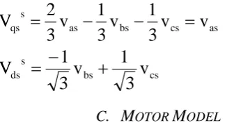
Here vossis zero-sequence convenient to set θ = 0 so that qs axis is aligned with as-axis. Therefore ignoring zero-sequence component, this can be simplified as-
as cs bs
as s
qs v v
3 1 v 3 1 v 3 2
V = − − =
cs bs s ds v 3 1 v 3 1
V = − + 2.4
C. MOTOR MODEL
The two-phase equivalent diagram of three-phase induction motor with stator and rotor windings referred to d – q axes. The winding are spaced by 90o electrical and rotor winding α, is at an angle θr from the stator d-axis. It is assumed that the d axis is leading the q axis for clockwise direction of rotation of the rotor. If the clockwise phase sequence is d-q, the rotating magnetic field will be revolving at the angular speed of the supply frequency but counter to the phase sequence of the stator supply. Therefore the rotor is pulled in the direction of the rotating magnetic field i.e. counter clockwise, in this case. The currents and voltages of the stator and rotor windings are marked in figure [2.2]. The number of turns per phase in the stator and rotor respectively are T1 and T2. A pair of poles is assumed for this figure. But it is applicable with slight modification for any number of pairs of poles if it is drawn in terms of electrical degrees. Note that θr is the electrical rotor position at any instant, obtained by multiplying the mechanical rotor position by pairs of electrical poles. The terminal voltages of the stator and rotor windings can be expressed as the sum of the voltage drops in resistances, and rate of change of flux linkages, which are the products of currents and inductances.
from the above figure the terminal voltages are as follows,
Vqs = Rqiqs + p (Lqqiqs) + p (Lqdids) + p (Lqαiα) + p (Lqβiβ)
Vds = p (Ldqiqs) + Rdids + p (Lddids) + p (Ldαiα) + p (Ldβiβ)
Vα = p (Lαqiqs) + p (Lαdids)+ Rαiα + p (Lααiα) + p (Lαβiβ)
Vβ = p (Lβqiqs) + p (Lβdids) + p (Lβαiα) + Rβ iβ + p (Lββiβ)
Where p is the differential operator d/dt, and vqs, vds are the terminal voltages of the stator q axis and d axis. Vα, Vβ are the voltages of
rotor α and β windings, respectively. iqs and ids are the stator q axis and d axis currents, respectively. iα and iβ are the rotor α and β windings currents, respectively. Lqq, Ldd, Lαα and Lββ are the stator q and d axis winding and
rotor α and β winding self-inductances, respectively.
The following are the assumptions made in order to simplify the equation
1. Uniform air-gap
2. Balanced rotor and stator winding
with sinusoidal distributed mmf.
3. Inductance in rotor position is
sinusoidal and
4. Saturation and parameter changes are neglected
From the above assumptions the equation modified as
vqs = (Rs + Ls p)iqs + Lsr p(iα sinθr) – Lsr p(iβ cosθr)
vds = (Rs + Ls p)ids + Lsr p(iα cosθr ) + Lsr p(iβ sinθr)
vα = Lsr p (iqs sinθr) + Lsr p (ids cosθr) + (Rrr + Lrrp)iα
vβ = - Lsrp (iqscosθr) + Lsr p (ids sinθr) + (Rrr + Lrrp)iβ
Where
Rs =Rq =Rd and
β α =
=R R
The rotor equations in above equation 2.8 refereed to stator side as in the case of transformer equivalent circuit. From this, the physical isolation between stator and rotor d-q axis use eliminated.
r o
θ Derivative of θr, a = transformer ratio = (stator turns)/(rotor turns)
rr 2
r a R
R = ; rr
2
r a L
L =
a i
iqr = qrr ;
a
i
i
dr=
drrvqr = avqrr ; vdr = avdrr
Magnetizing and control inductances are
2 1
m T
L α LsrαT1T2 Magnetizing inductance of the stator is
sr
m aL
L = 2.11
From equations 2.9, 2.10 &2.11 the equation 2.8 is modified as
+ θ θ θ − + θ − + + = dr qr ds qs r r r o r m r o m r o r r r r o m m m s s rrr s s dr qr ds qs i i i i p L R L p L L L p L R L p L p L 0 p L R 0 0 p L 0 p L R V V V V
Where θo
r = ωr = dθ/dt and p= d/dt
The dynamic equations of the induction motor in any reference frame can be represented by using flux linkages as variables. This involves the reduction of a number of variables in the dynamic equations. Even when the voltages and currents are discontinuous the flux linkages are continuous [12]. The stator and rotor flux linkages in the stator reference frame are defined as
ds m dr r dr qs m qr r qr dr m ds s ds qr m qs s qs i L i L i L i L i L i L i L i L + = + = + = + = ψ ψ ψ ψ ) ( ) ( dr ds m dm qr qs m qm i i L i i L + = + = ψ ψ qr dr r qr r qr dr qr r dr r dr qs qs s qs ds ds s ds p i R v p i R v p i R v p i R v ψ ψ ω ψ ψ ω ψ ψ + − = + + = + = + = 2.
Since the rotor windings are short circuited, the rotor voltages are zero. Therefore
0 0 = + − = + + qr dr r qr r dr qr r dr r p i R p i R ψ ψ ω ψ ψ ω r dr r qr qr r qr r dr dr R p i R p i ψ ω ψ ψ ω ψ + − = − − =
ψds =
∫
(vds −Rsids)dtdt
i R vqs s qs qs =
∫
( − )ψ r r r ds m qr r r dr sL R R i L L + + − = ωψ ψ r r qs r m dr r r qr sL R i R L L + + = ωψ ψ + − + = ) .( . s s r m dr s s ds ds sL R L sL sL R v i ψ + − + = ) .( . s s r m qr s s qs qs sL R L sL sL R v i ψ 2.22
The electromagnetic torque of the induction motor in stator reference frame is given by
e Lm iqsidr idsiqr
p
T = ( −
2 2 3
)
or 3 ( )
2 2
m
e qs ds ds qs r
L p
T i i
L ψ ψ
= −
The electro-mechanical equation of the induction motor drive is given by
dt d J p T
Te L r
ω 2 =
−
Mathematical modelling of induction motor III.
PID CONTROL THEORY
Zeigler-Nichols proposed rules for determining values of the proportional gain, integral time, and derivative time base on transient response characteristics of a given plant. Such determination of parameters of PID controllers can be made by engineers on site by experiments on plants. There are two methods of Ziegler Nichols tuning rules. In both the methods, they aimed at obtaining 25% maximum overshoot in step response. If the plant involves neither integrator(s) nor denominator complex conjugate poles, then such unit step response curve may look like an S-shaped curve, as shown. Such step response curves may be generated experimentally or from a dynamic simulation of the plant.
The S-shaped curve may be characterized by two constants, delay time L and time constant T. the delay time and time constant are determined by drawing a tangent line at the inflection point of the S-shaped curve and determining the intersections of the tangent line with the time axis and line c(t) = K. The transfer function C(S)/U(S) may then be
approximated by a first order system with a transport lag as follows
.
IV. PWM
CONTROL
Rise Timeis the time taken by asignalto change
from0% and 100% of the step height for under
damped system.
2 1
2
1 tan
1
n RiseTime
ς π
ς
ω ς
− −
− =
−
Peak Time is the time required for the response to
reach the peak overshoot.
2
1
n
PeakTime π
ω ς
= −
Settling Time is the time required for the response
to reach and stay at a specified tolerance band of its
final value.
ln(% )
n
error SettlingTime
ζω
=
Peak Overshoot is normalized difference between
the time responses peak and steady % is defined is
( Re ) ( ) ( )
C Peak sponse C PeakOvershoot
C
− ∞ =
∞
V. SIMULATION AND RESULTS
Fig.1 Final Simulink block diagram of Induction motor
Fig.2 Current Ouput for PID controlled Induction motor
Fig.4 Ouput Speed for PID controlled Induction motor
Fig.5 Current Ouput for PWM controlled Induction motor
Fig.6 Ouput electromagnetic torque for PWM controlled Induction motor
Fig.7 Ouput Speed for PWM controlled Induction motor
Fig.8 Current Ouput for cascaded controlled Induction motor
Fig.9 Ouput electromagnetic torque for cascaded controlled Induction motor
Fig.10 Ouput Speed for cascaded controlled Induction motor
Comparison of rise time, peak overshoot, peak time, settling time
Controller Rise time (seconds)
Peak Overshoot
(%)
Peak Time (%)
Settling time (seconds)
PI 5.88e-5 18.3 0.00203 0.012
PID 3.93e-5 27 0.0016 0.10
Cascaded 2.86e-5 157 0.0296 0.1776
CONCLUSION
Implementation of a modular Simulink model for induction machine simulation has been introduced .Unlike most other induction machine model implementations, with this model the user has access to all internal variables for getting an insight into the machine operation .any machine control algorithm can be simulated in the simulink environment with this model without actually using estimators .if need be ,when the estimators are developed, they can be verified using the signals in the machine model. The ease of implementation controls with this model is also demonstrated with several examples. Finally, the operation of model to simulate both the induction motors and generators has been shown so that there is no need for different models for different applications. When compared to v/f control method indirect vector control method is more reliable for its improved and better characteristics.
REFERENCES
[1] H. Inaba, S. Shima, A. Ueda, T. Ando, T. Kurosawa and Y. Sakai, "A new speed control system for DC motors usingGTO converter and its application to elevators," IEEE Trans. Ind. Applcat., vol. 21, pp. 391 -397, March/April 1985.
[2] M. Hombu, S..Ueda, A. Ueda and Y. Matsuda"A new current source GTO inverter with sinusoidal output Voltage and current," IEEE Trans. Ind. Applcat., vol. 2 1, pp. 1192-1 198, Sept./Oct. 1985. [3] H. Inaba, S. T. Nara, H. Takahashi$M. Nakazato,
"High speed elevators controlled by current source inverter system with sinusoidal input and output," Elevator World, pp. 54-60, March 1989.
[4] J. M. D. Murphy and F. G. Tumbull, Power Electronic control of AC motors, Pergamon Press, Oxford, England, 1988, pp. 306-330.
[5] Universal power analyzer PM 3000A users' manual, Voltech Instruments, Abingndon, England,
1997.
[6] S.K.Sul and T.A.Lipo, “Design and performance of a digitally based voltage controller for correcting phase,” IEEE Trans on Ind. Appl., vol.26, no.3, pp. 434-440, May/June, 1990
[7] R. Uhrin and F. Profumo, “Stand alone AC/DC converter for multiple inverter applications,” Power Electronics Specialists
Conference, PESC '96 Record, 27th Annual IEEE, Vol. 1, pp. 120 – 126, 23-27 June, 1996
[8] B. T. Ooi, Y.Guo, X.Wang, H.C. Lee, H.L. Nakra, and J.W. Dixon, “Stability of PWM HVDC Voltage Regulator Based on Proportional-Integral Feedback,” EPE Firenze’91, vol.3, pp.3-076-3-081, 1991
[9] M. Nishimoto, J.W. Dixon, A.B. Kulkarni and B.T. Ooi, “An integrated controlled-current PWM rectifier chopper link for sliding mode position control,” IEEE, Ind. Appl. Soc. Annual Meeting, pp. 752-757, October,
1996