Electronic Thesis and Dissertation Repository
10-25-2012 12:00 AM
Volatility, Duration, and Value-at-Risk
Volatility, Duration, and Value-at-Risk
Pujun Liu
The University of Western Ontario Supervisor
John Knight
The University of Western Ontario
Graduate Program in Economics
A thesis submitted in partial fulfillment of the requirements for the degree in Doctor of Philosophy
© Pujun Liu 2012
Follow this and additional works at: https://ir.lib.uwo.ca/etd
Part of the Econometrics Commons
Recommended Citation Recommended Citation
Liu, Pujun, "Volatility, Duration, and Value-at-Risk" (2012). Electronic Thesis and Dissertation Repository. 933.
https://ir.lib.uwo.ca/etd/933
This Dissertation/Thesis is brought to you for free and open access by Scholarship@Western. It has been accepted for inclusion in Electronic Thesis and Dissertation Repository by an authorized administrator of
(Spine title: Volatility, Duration, and Value-at-Risk) (Thesis format: Integrated Article)
by
Pujun Liu
Graduate Program in Economics
SUBMITTED IN PARTIAL FULFILLMENT OF THE REQUIREMENTS FOR THE DEGREE OF
DOCTOR OF PHILOSOPHY
SCHOOL OF GRADUATE AND POSTDOCTORAL STUDIES THE UNIVERSITY OF WESTERN ONTARIO
LONDON, CANADA OCTOBER 2012
c
CERTIFICATE OF EXAMINATION
Supervisor Examiners
Dr. John Knight Dr. Dinghai Xu
Supervisory Committee
Dr. Hao Yu
Dr. Youngki Shin Dr. Tim Conley
Dr. Martijn Van Hasselt Dr. Youngki Shin
The thesis by
Pujun Liu
entitled
Volatility, Duration, and Value-at-Risk
is accepted in partial fulfillment of the requirements for the degree of
Doctor of Philosophy
Date
Chair of the Thesis Examining Board
The thesis consists of three essays dealing with the modeling of volatility in financial markets, trade durations, and Value-at-Risk (VaR). The first essay models nonlinearities in the return series to estimate time-varying volatility by incorporating both regime changes and jumps. Two types of regime-switching GARCH-jump models with autoregressive jump intensity are presented. The first model follows the traditional Markov regime-switching model proposed in Hamilton (1989). As the unknown regimes in the Markov model lead to difficulty in forecasting, a threshold GARCH-jump model, in which regimes are known after observing the threshold variable in the previous period, is also proposed. The second essay models the intraday durations between two adjacent trade transactions by considering the impact of unaccounted struc-tural changes on parameter estimates. Monte Carlo simulations show that the observed high persistence in trade durations can be spurious and caused by unaccounted structural changes in the data generating process. The third essay investigates the use of realized moments in VaR forecasting, which is an important issue in risk management. Many VaR models rely only on the mean and volatility and ignore higher moments of returns, which leads to un-derestimation of VaR due to the unaccounted fat-tail property of the return series. Applying the Cornish-Fisher expansion to incorporate realized higher moments constructed from high frequency data, the proposed realized moment models outperform the realized volatility model and the traditional RiskMet-rics model, especially during the financial crisis period (2008-09).
It is an absolute pleasure to thank all the people who made this thesis possible.
First and foremost, I wish to express my deepest gratitude to my supervisor, Professor John Knight, for his continuous support of my Ph.D study and re-search, for his patience, encouragement, enthusiasm, as well as his immense knowledge and research experience. His dedication to research and students has taught me a lot about both work and life.
I would like to thank Youngki Shin and Martijn van Hasselt for being members of my committee and giving valuable suggestions to my papers and research. I would also like to thank Dinghai Xu for providing data used in the thesis, as well as his useful comments. My sincere thanks also goes to Lance Lochner, Maria Ponomareva, Yvonne Adams, Audra Bowlus, Chris Robinson, Hiroyoki Kasahara, Tim Conley, Peter Streufert, Yufeng Wang, Jin Zhou, Chris Mitchell and Yao Li.
Finally, I would like to thank my parents for their deepest love and continuous support throughout my life.
London, Canada Pujun Liu
August 12th, 2012
Certificate of Examination ii
Abstract iii
Acknowledgements iv
Table of Contents vi
List of Tables vii
List of Figures ix
List of Appendices xi
1 Introduction 1
1.1 Bibliography . . . 6
2 Regime-Switching GARCH-Jump Models with Autoregressive Jump Intensity 7 2.1 Introduction . . . 7
2.2 Markov Regime-Switching GARCH-Jump (RSGARJI) Model . . . 12
2.2.1 ARJI model by Chan and Maheu (2002) . . . 14
2.2.2 Construction of Markov Regime-Switching GARCH-Jump Model (RSGARJI Model) . . . 17
2.2.3 Properties of the Model with Exogenous Regime and an Estimation Mechanism . . . 20
2.3 Threshold GARCH-Jump model with Exogenous Trigger . . . 24
2.3.1 Model . . . 24
2.3.2 Stationarity Conditions and Moments of Returns . . . 27
2.5 Forecasting . . . 33
2.6 Conclusion . . . 42
2.7 Bibliography . . . 45
3 Autoregressive Conditional Duration Models with Structural Changes 48 3.1 Introduction . . . 48
3.2 Literature Review . . . 51
3.3 The ACD Framework . . . 53
3.4 Monte Carlo Simulation . . . 56
3.4.1 Individual Shift in the Intercept Parameterω. . . 56
3.4.2 Individual Shift inα . . . 60
3.4.3 Individual Shift inβ . . . 62
3.5 Theoretical Results . . . 63
3.6 Threshold ACD model and Empirical Estimation . . . 65
3.7 Conclusion . . . 72
3.8 Bibliography . . . 74
4 Value-at-Risk Estimation via Realized Higher Moments using High Frequency Data 77 4.1 Introduction . . . 77
4.2 VaR via Cornish-Fisher Expansion . . . 82
4.3 Realized Moments Measurement . . . 83
4.3.1 Realized Moments Model to Calculate VaR . . . 83
4.3.2 Data and Empirical Properties of Realized Moments . . . 86
4.4 Realized Moment Forecasting Models . . . 102
4.4.1 RM-EWMA Model . . . 102
4.4.2 RM-ARFIMA Process . . . 106
4.5 Empirical Results . . . 108
4.5.1 Data Sampling . . . 108
4.5.2 Realized Volatility Incorporating Overnight Information . 109 4.5.3 Realized Moments Forecasting Results . . . 111
4.5.4 Statistical Evaluation . . . 116
4.5.5 VaR Forecasting Results . . . 117
4.6 Conclusion . . . 121
4.7 Bibliography . . . 126
A Proof of Proposition 2.1 134 B Proof of Proposition 2.2 136 C Proof of Proposition 3.1 140
Curriculum Vitae 143
2.1 Descriptive Statistics of Daily Returns of Japanese Yen . . . 29 2.2 Estimates and log likelihood values using different models . . . . 31 2.3 Out-of-sample evaluation statistics of conditional variance
fore-casts . . . 38
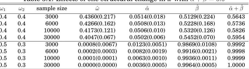
3.1 Effects of one structural change inωwithα+β= 0.6 . . . 58 3.2 Simulation results of a temporary change inωwithα+β = 0.6 . 60 3.3 Simulation results of a permanent change inα(ω= 0.1andβ = 0.6) 61 3.4 Simulation results of a temporary change inα(ω = 0.1andβ = 0.6) 62 3.5 Simulation results of a permanent change inβ(ω = 0.1andα= 0.1) 63 3.6 Effects of a temporary change inβ (ω= 0.1andα = 0.1) . . . 63 3.7 Estimation results of exponential ACD model and exponential
TACD model . . . 72 3.8 Estimation results of Weibull ACD model and Weibull TACD model 73
4.1 Summary statistics of daily IBM return . . . 88 4.2 Summary statistics for unconditional distributions of realized
volatil-ity, RM(3) and RM(4) . . . 90 4.3 Summary statistics for unconditional distributions of
transfor-mations of realized moments . . . 97 4.4 Test statistics oflnRM(4) . . . 98 4.5 Estimation Results for ARFIMA models oflnRV andlnRM(4) . 112 4.6 Lambdas and correlations of EWMA procedure . . . 116
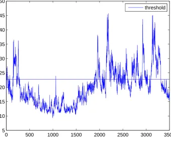
2.1 VIX with estimated threshold value for the threshold GARCH
model . . . 34
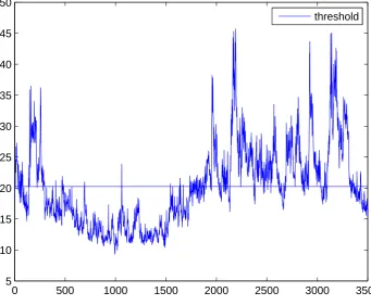
2.2 VIX with estimated threshold value for the threshold GARCH-jump model . . . 35
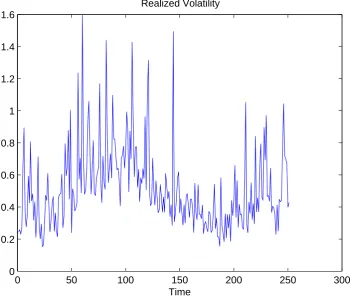
2.3 Out-of-sample realized volatility from Jan 2004 to Jan 2005 . . . 38
2.4 Out-of-sample conditional variance forecast using GARCH (1,1) model . . . 39
2.5 Out-of-sample conditional variance forecast using threshold-GARJI model . . . 40
2.6 Out-of-sample conditional variance forecast using Regime-switching GARJI model . . . 41
3.1 Adjusted duration from September 1, 2000 to October 31, 2000 . 68 3.2 Adjusted duration with sample size of 5000 . . . 69
3.3 Sample autocorrelation function of Boeing transaction durations from September 1, 2000 to October 31, 2000 . . . 70
4.1 Time series of IBM daily return . . . 88
4.2 Time series of IBM realized volatility . . . 91
4.3 Time series of IBM realized third moment . . . 92
4.4 Time series of IBM realized fourth moment . . . 93
4.5 Autocorrelations of IBM realized fourth moment . . . 96
4.6 Time series of logarithmic realized fourth moment, IBM . . . 97
4.8 Autocorrelations of IBM logarithmic realized fourth moment in
the pre-crisis period . . . 99
4.9 Autocorrelations of IBM logarithmic realized fourth moment in the crisis period . . . 100
4.10 Autocorrelations of IBM logarithmic realized fourth moment in the post-crisis period . . . 101
4.11 Autocorrelations of IBM realized third moment . . . 103
4.12 Time series of logarithmic realized volatility, IBM . . . 113
4.13 Autocorrelations of logarithmic realized volatility, IBM . . . 114
4.14 Normal quantile plot of residuals of ARFIMA model for IBM log-arithmic realized volatility . . . 122
4.15 Normal quantile plot of residuals of ARFIMA model for IBM log-arithmic realized fourth moment . . . 123
A Proof of Proposition 2.1 . . . 135 B Proof of Proposition 2.2 . . . 139 C Proof of Proposition 3.1 . . . 142
Chapter 1
Introduction
This dissertation consists of three essays dealing with the modeling of volatility
in financial markets, financial asset trade durations, and Value-at-Risk. The
thesis is related to both regularly spaced and irregularly spaced financial data.
Chapter 2 takes into consideration non-linearity issues in the return series to
estimate volatility by incorporating both regime changes and jumps.
Chap-ter 3 deals with irregularly spaced financial data by considering the impact
of unaccounted structural changes on parameter estimates of intraday trade
duration process. An important issue in risk management is the forecasting
of market Value-at-Risk (VaR). In Chapter 4, two new VaR forecasting
mod-els are proposed. Realized higher moments are constructed to provide better
VaR forecasts, taking advantage of the information conveyed in high frequency
data.
Jump Intensity, two types of regime-switching GARCH-jump models with
au-toregressive jump intensity are proposed to model the non-linearity in return
series and the associated volatility. Chan and Maheu (2002) present an
au-toregressive jump intensity model to explain the jump clustering phenomenon.
However, the forecasts of their model are inaccurate when the out-of-sample
period differs from the in-sample period in the frequency of jumps. To solve this
problem, regime shifts are incorporated in both the smoothly changing GARCH
term and the infrequent jump term. The first model is a Markov
regime-switching model which generalizes the GARCH model by distinguishing two
regimes with different GARCH volatility and jump intensity levels. As the
regimes are unknown to the econometrician in the Markov regime-switching
model, which leads to difficulty in forecasting, a threshold GARCH-jump model
with an exogenous threshold variable is also proposed. The stationarity
con-ditions and moments of returns are derived for the threshold GARCH-jump
model. Using Japanese YEN-US Dollar exchange rates, it is shown that both
types of regime-switching models have better performance than the traditional
GARCH model for the in-sample period. Constructing realized volatility from
5-minute intraday data for evaluation, the threshold GARCH-jump model
out-performs the single regime autoregressive jump intensity model to provide
volatility forecasts.
The rapid development in computer technology has led to the availability
traditional econometric techniques inapplicable. To solve this problem, Engle
and Russell (1998) build a linear autoregressive conditional duration (ACD)
model to account for stochastic clustering of durations between two adjacent
trades. In Chapter 3, Autoregressive Conditional Duration Models with
Struc-tural Changes, we find that high persistence of trade durations noted in the
literature, i.e., the sum of estimated autoregressive coefficients on lagged
du-rations and conditional expected dudu-rations are close to one, may come from
unaccounted structural shifts in the data generating process. Monte Carlo
ex-periments are conducted to show that even a temporary change in one
param-eter of the ACD model for a relatively short time period can lead to a big bias
in the estimates of the autoregressive parameters, which converge to one as
jump size increases. The sample mean of the conditional expected duration is
derived for ACD model with structural changes. Finally, we estimate Boeing
transaction duration data using a threshold ACD model and find that it fits the
data better than the single-regime ACD model.
Under the Basel II and Basel III Accords, banks are required to maintain
regulatory capital for market risk according to their assets’ riskiness, which is
defined as theα%VaR, such that the loss of a specific asset within a future time
period will only be surpassed for (1−α)% of the time. Many VaR models rely
only on the mean and volatility of the return series and ignore higher moments,
property of the return series. Aiming to solve this issue, Chapter 4,
Value-at-Risk Estimation via Realized Higher Moments using High Frequency Data,
investigates the impact of realized higher moments constructed from high
fre-quency data on VaR forecasts. Recently, Amaya et. al (2011) proved that,
un-der realistic assumptions of an affine jump-diffusion process with stochastic
volatility, the realized moments converge in mean square to the integrated
mo-ments up to the fourth moment. The well-known realized variance is a special
example of realized moments, i.e., it is the realized second moment. As
real-ized moments are ex post measures, two new models are proposed to provide
one-step-ahead forecasts for realized moments, after exploring the
characteris-tics of realized moments. We find that the logarithmic realized fourth moment
is significantly autocorrelated and often displays long memory properties. The
first model extends the exponentially weighted moving average (EWMA)
pro-cedure to realized volatility and the logarithmic realized fourth moment. The
second model applies an autoregressive fractionally integrated moving average
(ARFIMA) model to both the logarithmic realized volatility and logarithmic
re-alized fourth moment according to their autoregressive and long-memory
char-acteristics. After calculating skewness using forecasts of realized moments,
we apply the Cornish Fisher approximation to incorporate the time-varying
volatility and kurtosis in the VaR forecasting. In an empirical study, we
com-pare the performance of realized moments models with other VaR models such
the realized moments models provide accurate forecasts and outperform the
Riskmetrics model and the realized volatility model, especially during the
1.1
Bibliography
AMAYA, D., P. CHRISTOFFERSEN, K. JACOBS, AND A. VASQUEZ(2011): “Does
Realized Skewness and Kurtosis Predict the Cross-section of Equity
Re-turns?,”working paper.
CHAN, W., AND J. M. MAHEU (2002): “Conditional jump dynamics in stock
market returns,”Journal of Business&Economic Statistics, 20(3), 377–389.
ENGLE, R., AND J. RUSSELL (1998): “Autoregressive conditional duration: a
new model for irregularly spaced transaction data,”Econometrica, 66, 1127–
Chapter 2
Regime-Switching GARCH-Jump
Models with Autoregressive
Jump Intensity
2.1
Introduction
Estimating and forecasting volatility is an important task in financial markets.
Volatility, interpreted as uncertainty of return and calculated as the standard
deviation or variance of the return series, is a key variable in derivative
pric-ing, portfolio rebalancing and risk management. As it is widely perceived that
volatility of asset returns is changing over time, it is important to investigate
the characteristics of the volatility process.
Jump diffusion models are a class of volatility models which have received
wide-spread acceptance for their ability to model both continuous small changes
and infrequent large movements in financial return series since the seminal
diffusion models, GARCH models and stochastic volatility models are used
to account for the diffusion part in return, or the smoothly changing
move-ments that might be caused by normal news events as well as liquidity
trad-ing. Jumps refer to the infrequent large movements in return that are caused
by the unusual and important news events, such as earning surprises. For the
jump part, jump intensity, which refers to the arrival rate of jumps, is
usu-ally assumed to be independent, partly because of the difficulty of estimation
of stochastic jump intensity models without a closed-form likelihood function.
Recently, Chan and Maheu (2002) and Maheu and McCurdy (2004) model the
return series as a combination of jumps and smoothly changing components,
in which the conditional jump intensity is autoregressive. They find that the
jump intensity is strongly rejected to be constant. The autoregressive
parame-ter in the jump intensity is positively significant and high for individual stock
returns, which supports the phenomenon of jump clustering.
While jump diffusion models present a parametric way to model abnormal
or jump innovations as well as normal innovations, the harnessing of high
fre-quency data in the last decade has also led to separate analysis of diffusive
and jump components using a non-parametric approach. Daily realized
volatil-ity, constructed by Andersen and Bollerslev (1998) and Bandorff-Nielsen and
Shephard (2001) using the summation of squared intraday returns, is a
with a bounded jump intensity. This provides a good proxy for daily
volatil-ity after dealing with intraday pattern and microstructure noise. Moreover,
Bandorff-Nielsen and Shephard (2004) present realized bipower variation
con-structed from high frequency data, which is consistent for the integrated
vari-ance in the same jump-diffusion setting. As the difference of quadratic
varia-tion and the integrated variance is the cumulative squared jumps, the result
renders feasible statistical tests for the presence and impact of jumps. Huang
and Tauchen (2005) show that a test for jumps has good power and detection
capacities using Monte Carlo analysis, and indicate strong empirical evidence
for jumps to account for stock market price variance.
Another line of literature deals with non-linearity using regime switching
models. Lamoureux and Lastrapes (1990) show that the high persistence of
the conditional variance using GARCH model may be overstated due to the
failure of recognizing structural changes in the model. Gray (1996) develops
a generalized regime switching GARCH model and finds that it outperforms
single-regime models out-of-sample using short-term interest rate. More
re-cently, Hillebrand (2005) show that the convergence of the sum of estimated
autoregressive parameters holds for all common estimators of GARCH. Thus,
in the presence of neglected parameter changes, GARCH is no longer a suitable
model to measure persistence.
regime switching GARCH-jump models based on Chan and Maheu (2002)’s
au-toregressive jump intensity (ARJI) model. The motivation is that although the
ARJI model provides good in-sample estimation, the out-of-sample forecasting
ability is not as good especially when the jump frequency in the out-of-sample
period differs from the in-sample period. For example, when the out-of-sample
period is a relatively tranquil period which contains less jumps, using
param-eters estimated from the relatively volatile in-sample period will overestimate
the jump frequency and lead to inaccurate forecasting. In this chapter we show
that the out-of-sample forecasting performance is not as good as GARCH model
for Japanese Yen-US Dollar exchange rate. Thus, it is necessary to distinguish
between volatile period and tranquil period for jumps. In addition, Maheu and
McCurdy (2004) plot the time-series of conditional variance components of IBM
estimated by their generalized autoregressive jump intensity (GARJI) model,
in which both GARCH component and jump component of the conditional
vari-ance are higher than normal in some periods, while in other periods both of
them are less volatile. The phenomenon suggests that both smooth changes
and jumps may be governed by regime changes. Furthermore, the high
persis-tence in conditional variance may be spurious due to latent structural changes
in the data generating process. Thus, we model the GARCH volatility and jump
intensity process in different regimes in order to improve the out-of-sample
forecasting performance.
one follows the traditional Markov regime-switching model proposed in
Hamil-ton (1989), which has good stationarity conditions but latent regimes. The
diffi-culty to introduce regimes into conditional jump intensity in this type of model
is that the jump intensity will depend on the entire regime path from the
be-ginning of the period to the current period as it is autoregressive, which leads
to computational complexity. To circumvent this problem, the jump intensity is
assumed to depend only on its current regime state. However, since the regimes
are unknown this results in poor forecasting in the Markov regime-switching
models. Consequently, we also consider a threshold GARCH-jump model, in
which regimes are known after the observation of the threshold variable at the
previous period. Recently, Knight and Satchell (2011) derive sufficient and
nec-essary conditions for the existence of a stationary distribution for a threshold
AR (1) model with exogenous threshold variable. We extend their research and
find stationarity conditions for the threshold GARCH-jump model with regimes
in both GARCH type conditional variance and jump intensity.
The chapter is organized as follows. Section 2.2 presents the Markov
regime-switching GARCH-jump model and proposes an estimation mechanism after a
brief review of the ARJI model by Chan and Maheu (2002). In section 2.3, the
threshold GARCH-jump model with an exogenous trigger is developed and
sta-tionarity conditions are derived. Empirical analysis is conducted in sections
for the estimation, in which realized volatility constructed from 5-minute
intra-day data are used as proxy of volatility for evaluation of forecasts of different
models. Section 2.6 contains a brief conclusion.
2.2
Markov Regime-Switching GARCH-Jump
(RS-GARJI) Model
Regimes are incorporated into both GARCH variance and jump intensity. For
a Markov regime-switching GARCH (1,1) with jump intensity as an AR (1)
process, which is denoted by RSGARJI model, the model is given by
Rt=µ+ϵ1,t+ N(t) ∑
k=1
Yt,k
ϵ1,t =ztσt
Yt,k ∼i.i.d N(θ, δ2)
P(N(t) = j|Φt−1) = exp(−λt)λjt/j! for j= 0, 1, 2...
In regimest, forst= 1,2,
σt2 =ωst +astϵ
2
t−1+bstE[σ
2
λt=αst +ρstE[λt−1|Φt−1, st] +γstE[ξt−1|Φt−1, st] (2.2)
ξt−1 =E[N(t−1)|Φt−1, St−1]−λt−1
Rtdenotes the return at time t, which is the first difference of logarithmic price.
ϵ1,t is a GARCH component with an autoregressive conditional varianceσ2t, and ∑N(t)
k=1 Yt,k is the jump innovation which is a compound Poisson process. As in
the GARCH model, zt follows the normal distribution with mean 0 and
vari-ance 1. The GARCH component can explain the continuous small changes in
the return series. N(t)is the number of jumps happening at time t, which
fol-lows a Poisson process with autoregressive jump intensity λt. Jumps happen
occasionally. If N(t) = 0, there is no jumps at time t. So, the jump
innova-tion, can explain for the infrequent large movements in the return series. st
denotes the regime at time t, which can take value of 1 or 2 referring to two
different regimes. St is the entire regime path {st, st−1, ...}. Φt−1 denotes the
information set until time t −1. Smoothly changing components are
repre-sented by ϵ1,t, which follows a GARCH process with different parameters in
different regimes, corresponding to (ωst, ast, bst)in regime st. The jump
inten-sityλt follows an approximate AR(1) process in each regime, with parameters
(αst, ρst, γst) in regime st. We use the approximate AR(1) process introduced
the problem that the likelihood function has no closed form when the jump
in-tensity follows an ARMA process. ξt−1 can be viewed as an approximate error
term. It will be discussed later.
When regimes are assumed to be exogenous, i.e, explanatory variables in
the conditional intensity processσtcontain no information aboutstbeyond that
contained inΦt−1,stfollows a first-order Markov process as in Hamilton (1989).
P(st=j|St−1) = P(st =j|st−1 =i) = pij (2.3)
The transition matrix is
P =
[
p11 1−p11
1−p22 p22 ]
p11andp22 are respectively the persistence of regime 1 and regime 2.
This is the model setting when the regimes follows a Markov process. In
the following subsections, we discuss why the model is built this way. First we
present the autoregressive jump intensity (ARJI) model of Chan and Maheu
(2002) and discuss its properties. Then we elaborate on the way of constructing
the regime-switching model in both conditional variance and jump intensity.
2.2.1
ARJI model by Chan and Maheu (2002)
Previous literature suggests that jump intensity is time-varying and may
de-pend on its lagged values. For example, Knight and Satchell (1998) model
stochastic deviation from fundamentals. By substitution the jump intensity
can be expressed as an autoregressive form together with non-negative error
term. Chan and Maheu (2002) and Maheu and McCurdy (2004) generate an
autoregressive conditional jump intensity (ARJI) model and derive conditional
moments of the returns. In applications to several individual firms, the
per-sistence parameter for the arrival of jump events is quite high, up to 0.924 for
Texaco. Their model is a single-regime discrete-time GARCH-jump model with
time dependent jump intensity with the following specification.
λt =α+ρλt−1+γξt−1
ξt−1 =E[N(t−1)|Φt−1]−λt−1
E[N(t − 1)|Φt−1] is the ex post assessment of the expected number of jumps
given information set Φt−1, while λt−1 is the ex ante assessment. So ξt can
be viewed as the change in the conditional forecast of the jumps after the
infomation set is updated. It is a martingale difference sequence with
re-spect to {Φt−1}, as E[ξt−1|Φt−2] = E[E[N(t−1)|Φt−1]−E[N(t−1)|Φt−2]|Φt−2] =
E[N(t− 1)|Φt−2] −E[N(t− 1)|Φt−2] = 0, which implies that there is no
auto-correlation in the intensity residual and the unconditional expectation is zero.
Thus it can be viewed as an error term in the jump intensity process. If|ρ|<1,
then the jump intensity is covariance stationary. The conditional mean of
σ2
t + (θ2 +δ2)λt, which is a combination of the GARCH conditional variance
component and the jump component.
Maheu and McCurdy (2004) describe some empirical results found by the
model. They find strong evidence of time dependence in jump intensities for
both stock indices and several individual stocks. The average proportion of
conditional variance explained by jumps varies from 20% to 40%, at times as
much as90%. It is much higher than Huang and Tauchen (2005)’s finding that
jumps account for 7 percent of stock market price variance usingS&P index.
The ARJI model provides better out-of-sample forecasts following large
neg-ative moves in the market. However, the forecasts may be worse than the
GARCH (1,1) model when the out-of-sample period differs with the in-sample
period in frequency of jumps. As jumps are infrequent and hard to predict,
there is no reason to assume that the out-of-sample period has similar
fre-quency of jumps as the in-sample period. When the in-sample period has a
relatively lower jump intensity than the out-of-sample period, the forecasts of
volatility based on the in-sample parameters will be underestimated. Thus, it’s
2.2.2
Construction of Markov Regime-Switching
GARCH-Jump Model (RSGARJI Model)
The reported high persistence of conditional variance by GARCH models,
to-gether with high level of jump clustering revealed in Maheu and McCurdy
(2004), may be spurious and due to structural shifts in the data generating
process, such as deterministic changes in the intercept parameter of
autore-gressive jump intensity process. What’s more, there are periods during which
few jumps happen and other periods when jumps cluster. In an attempt to
solve the problem, we now introduce regime shifts into the conditional jump
intensity. To incorporate structural changes in the data generating process, a
popular approach is the Markov regime-switching model applied to dependent
processes by Hamilton (1989). State 1 and state 2 refer to low jump intensity
regime and high jump intensity regime respectively, and a Markov process is
used to govern the switches between regimes. The jump intensity depends on
its own lagged value within each regime.
The regime-switching model is based on ARJI model for two reasons. Firstly,
the autoregressive jump intensity setting can account for clustering of jumps
and also incorporate shocks. By introducing regimes into GARCH-type
condi-tional variance and jump intensity, we can explore if persistence of condicondi-tional
variance and jumps vary for different regimes and whether the high
persis-tence is spurious due to structural changes. Secondly, jump diffusion models
has no closed form. The ARJI model avoids this problem by assuming
approx-imate autoregressive jump intensity structure with a filter to infer the ex post
distribution of jumps.
Let {st} be a Markov Chain with 2-dimensional state space. In state 1,
jumps are not so frequent, while jumps are more likely to happen in state 2. St
denotes the regime path at time t,{st, st−1, st−2, ...}. Φt−1 refers to the
informa-tion set at time t−1. To clarify, ϵt refers toRt−µ, which is the summation of
ϵ1,t and the jump part.
The first specification for the conditional jump intensityλtis
P(N(t) =j|Φt−1, St, xt) = exp(−λt)λ j
t/j! forj = 0,1,2... (2.4)
λt =α1+ρ1λt−1+γ1ξt−1 ifst= 1 (2.5)
λt =α2+ρ2λt−1+γ2ξt−1 ifst= 2 (2.6)
The conditional jump intensity, λt = E(N(t)|Φt−1, St), has an autoregressive
form and depends on contemporaneous conditional variance and trading
vol-ume. Hereby ξt−1 = E[N(t −1)|Φt−1, St−1] −λt−1, which also depends on the
state space of regimes. It is easy to show that ξt is still a martingale
differ-ence sequdiffer-ence with respect to{Φt−1, St−1}, whereΦt−1 is the information set up
to t−1,which is composed of past values of Rt. Therefore it is a well defined
However, this specification for jump intensity has computational
difficul-ties. Although the current regime only determines the parameters α,ρ and γ,
the dependence ofλton both the current regime and its own lagged valueλt−1
makes λt depend on the entire regime path{st, st−1, st−2, ...}, by iterative
sub-stitution. As the regimes are latent, the inability to observe them leads to the
need of integrating out all possible paths when calculating the sample
likeli-hood. It makes the estimation practically intractable. This problem is similar
to that which arises in regime-switching GARCH models, as noted by Klaaseen
(2002), which models the GARCH type volatility as a regime-switching process.
To circumvent the problem of path dependence, we model the conditional
jump intensity as
λt=αst +ρstE[λt−1|Φt−1, st] +γstE[ξt−1|Φt−1, st] (2.7)
where λt = E[N(t)|Φt−1, st]. Note that λt depends only on st instead of St now.
The idea is inspired by Klaaseen (2002) to integrate out the regime path St−1
out of the right hand side of the equation. After St−1 is integrated out for
conditional intensity of the last period, the right hand side only depends on
the current regimest. In addition, this is equivalent to integrating outst−1,the
regime at timet−1, as the lag of equation (2.7) implies thatλt−1 only depends
on st−1 and is independent of St−2. st is included in the conditioning variables
because it may contain some information about the last period regimest−1.
In order for λt to be positive for all t, a sufficient condition is that αst > 0,
removes the problem of regime path dependence, and allows the jump intensity
to be autocorrelated, which can help explain the phenomenon of jump
cluster-ing around significant news events.
2.2.3
Properties of the Model with Exogenous Regime and
an Estimation Mechanism
The steady state probabilities of the regimes 1 and 2 at timet−1,P(st−1 = 1)
andP(st−1 = 2), are derived in Hamilton (1989),
P(st−1 = 1) =
1−p22 2−p11−p22
(2.8)
P(st−1 = 2) =
1−p11 2−p11−p22
(2.9)
Proposition 2.1. If the unconditional jump intensity exists for both regime 1 and 2, denoted byλ1 and λ2 respectively, then
λ1
λ2
=B−1
α1
α2 (2.10) with B =
1−ρ1p11 −ρ1(1−p11) −ρ2(1−p22) 1−ρ2p22
(2.11)
The proof of Proposition 2.1 is in Appendix A. From Proposition 2.1, for the
existence of the unconditional jump intensity, the inverse of B , the
the unconditional jump intensity to be strictly positive for all t, the four
ele-ments of the inverse ofB should be positive.
B−1 = 1
1−ρ1p11−ρ2p22−ρ1ρ2(1−p11−p22) [
1−ρ2p22 ρ1(1−p11)
ρ2(1−p22) 1−ρ1p11 ]
(2.12)
For the unconditional jump intensity to be strictly positive, 1−ρ1p11−ρ2p22−
ρ1ρ2(1−p11−p22)>0,1−ρ1p11 >0, and1−ρ2p22>0.
Then the conditional variance ofRtis
V ar(Rt|Φt−1) = ∑
st=1,2
P(st|Φt−1)V ar(Rt|st,Φt−1)
= ∑
st=1,2
P(st|Φt−1)(σ2t + (θ
2+δ2)λ
t) (2.13)
The estimation of the model can be conducted by maximum likelihood based
on the estimation mechanism of the ARJI model using an iterative algorithm.
As there are two latent variables, the regime variable stand number of jumps
Nt, the conditional density function is computed by integrating out the regime
variable and number of jumps step by step.
f(Rt|Φt−1) = f(Rt|Φt−1, st= 1)P(st = 1|Φt−1) +f(Rt|Φt−1, st= 0)P(st= 0|Φt−1)
= [ ∞
∑
j=0
f(Rt|N(t) = j,Φt−1, st = 1)P(N(t) =j|Φt−1, st)]P(st= 1|Φt−1)
+ [ ∞
∑
j=0
f(Rt|N(t) = j,Φt−1, st = 0)P(N(t) =j|Φt−1, st)]P(st= 0|Φt−1)
(2.14)
When there is an infinite summation in the likelihood function, I truncate it
the tail of the conditional Poisson distribution for jump numbers larger than
15, which is in accordance with Maheu and McCurdy (2004)’s finding. The
first part of the right hand side of the conditional sample likelihood function,
f(Rt|N(t) = j,Φt−1, st),can be derived as follows. Note that σ2t depends onst.
f(Rt|N(t) =j,Φt−1, st) =
1 √
2π(jδ2 +σ2 t)
exp(−(Rt−µ−jθ) 2
2(jδ2+σ2 t)
) (2.15)
Then the expression ofP(N(t) = j|Φt−1, st)andP(st|Φt−1)is needed.
From the model specification, it’s known that
P(N(t) =j|Φt−1, st) = exp(−λt)λ j
t/j! forj = 0,1,2... (2.16)
whereλtis a function ofst, which is not straightforward to compute because of
integrating out of regime pathSt−1 inE[λt−1|Φt−1, st].
λt=αst +ρstE[λt−1|Φt−1, st] +γstE[ξt−1|Φt−1, st] (2.17)
Asλt−1 is a function ofst−1,
E[λt−1|Φt−1, st] = ∑
st−1=1,2
λt−1(st−1)P(st−1|Φt−1, st) (2.18)
ξt = E[N(t)|Φt, st]−λt is also a function of st. The density of the expectation
part ofξtis
P(N(t) =j|Φt, st) =f(Rt|N(t) =j,Φt−1, st)P(N(t) = j|Φt−1, st)/f(Rt|Φt−1, st)
(2.19)
Then
ξt−1 = ∞
∑
j=0
E[ξt−1|Φt−1, st] = ∑
st−1=1,2
ξt−1(st−1)P(st−1|Φt−1, st) (2.21)
After getting P(st|Φt−1) and P(st−1|Φt−1, st), the sample likelihood can be
re-solved. According to Bayes’ rule,
P(st−1|Φt−1, st) =
P(st−1|Φt−1)P(st|st−1,Φt−1)
P(st|Φt−1)
(2.22)
P(st|Φt−1) = ∑
st−1=1,2
P(st|st−1,Φt−1)P(st−1|Φt−1) (2.23)
where P(st|st−1,Φt−1) = P(st|st−1) is the transition probability. The
computa-tion of ex post regime probability P(st−1|Φt−1) and ex ante regime probability
P(st|Φt−1) is discussed in Hamilton (1994) and works by applying a first-order
recursive mechanism. That is,
P(st−1|Φt−1) =
f(Rt−1|st−1,Φt−2) ∑
st−2=1,2(P(st−2|Φt−2)P(st−1|st−2,Φt−2))
f(Rt−1|Φt−2)
(2.24)
and
f(Rt−1|st−1,Φt−2) = ∞
∑
j=0
f(Rt−1|N(t−1) = j,Φt−2, st−1)P(N(t−1) =j|Φt−2, st−1)
(2.25)
Thus, the iterative procedure is as follows:
Step 1. Set the initial values of P(s0|Φ0), σ02 and λ0 as their unconditional means respectively. ξ0 is set to be 0.
Step 2. Given P(s0|Φ0), P(s1|Φ0) is computed using equation (2.23), which is then used to calculateP(s0|Φ0, s1)via equation (2.22).
used to calculate f(R1|N(1) = j,Φ0, s1)using equation (2.15). Together with λ1
derived from equation (2.17),f(R1|Φ0)can be computed using equation (2.14).
Step 4. f(R1|Φ0, s1) is derived via equation (2.25). Consequently, P(N(1) =
j|Φ1, s1) is available with equation (2.19), and P(s1|Φ1) is derived from
equa-tion (2.24). Together with the value of λ1, E[ξ1|Φ0, s1] and E[λ1|Φ0, s1] can be
computed. Then λ2 is available to compute the density f(R2|Φ1). The sample
likelihood can be computed using this iterative procedure.
As the log likelihood function has a closed form expression, maximum
like-lihood method can be applied to estimate the model when the regime variable
is exogenous.
2.3
Threshold GARCH-Jump model with
Exoge-nous Trigger
2.3.1
Model
One main shortcoming of the hidden Markov regime switching model,
dis-cussed in the last section, is that the regimes of each period are not known
to the econometrician, and this leads to difficulty with forecasting, especially
when used to forecast volatility a few days later. Threshold models with
ob-servable triggers can solve this problem. In threshold models, when the trigger
otherwise. Thus, in each period, the regime can be observed, which is an
exoge-nous variable. While estimation of threshold models poses no difficulty, there
are limited theoretical results available concerning the stationarity conditions,
and existence of moments.
Recently, Knight and Satchell (2011) derived necessary and sufficient
con-ditions for the existence of a stationary distribution of threshold-AR (1) model
with an exogenous trigger variable. As our GARCH-jump model is a GARCH
model with AR (1) jump intensity, these conditions for the threshold-AR (1) can
be applied to the threshold GARCH-jump model with an exogenous trigger.
The threshold GARCH-jump model is
Rt=µ+ϵ1,t+ N(t) ∑
k=1
Yt,k (2.26)
ϵ1,t =ztσt (2.27)
Yt,k ∼N.I.D(θ, δ2) (2.28)
P(N(t) = j|Φt−1) = exp(−λt)λjt/j! forj = 0,1,2... (2.29)
λt=α1+ρ1λt−1+γ1ξt−1 ifνt−1 ≤ν0 (2.31)
ξt−1 =E[N(t−1)|Φt−1]−λt−1 (2.32)
σt2 =ω2+a2ϵ2t−1+b2σt2−1 ifνt−1 > ν0 (2.33)
λt=α2+ρ2λt−1+γ2ξt−1 ifνt−1 > ν0 (2.34)
Φt−1 denotes the information up to timet−1, which includes the time series of
Rtand threshold variableνtup to timet−1. In this model setting, there are two
regimes as well as in the previous hidden Markov regime-switching model. The
parameters in the GARCH conditional variance and jump intensity depends on
the threshold variableνt. In hidden Markov model regimes in each period are
unknown to the econometricians both before and after the estimation, however,
in the threshold model the regimes are known to the econometrician, which is
very helpful in the estimation as well as in forecasting. For example, there is
no need to integrate out the previous regimes in the threshold model, which
simplifies the estimation algorithm. Let st = 0 ifνt ≤ ν0, and st = 1ifνt > ν0,
where we assume thatst follows a i.i.d Bernoulli distribution withP(st= 1) =
2.3.2
Stationarity Conditions and Moments of Returns
Proposition 2.2. λtis strictly stationary ifln|ρ1|(1−π)+ln|ρ2|π <0. The return
series is covariance-stationary if |ρ1|(1−π) +|ρ2|π < 1 and |(a1 +b1)|(1−π) +
|(a2+b2)|π <1. The mean of return is given by
E(Rt) = µ+θE(λt) = µ+θ(
α1(1−π) +α2π 1−ρ1(1−π)−ρ2π
)
The variance of return is given by
V ar(Rt) =
ω1(1−π) +ω2π
1−(a1+b1)(1−π)−(a2+b2)π
+ (θ
2+δ2)(α
1(1−π) +α2π)(1−b1(1−π)−b2π) (1−ρ1(1−π)−ρ2π)(1−(a1+b1)(1−π)−(a2+b2)π)
The proof of Proposition 2.2 is in Appendix B. It shows that both the mean
and the variance of return depends on the parameters and probability of each
regime. The conditional skewness and kurtosis are given by
Skewness(Rt|Φt−1) =
λt(θ3+ 3θδ2) (σ2
t +λtδ2t +λtθ2)3/2
(2.35)
Kurtosis(Rt|Φt−1) = 3 +
λt(θ4+ 6θ2δ2+ 3δ4) (σ2
t +λtδ2+λtθ2)2
(2.36)
The derivation of the above conditional moments is given in Das and
Sun-daram (1997). The skewness is positive if θ > 0. Both skewness and kurtosis
depend on the conditional jump intensity λt, the jump size’s mean θ and
vari-anceδ2. The conditional kurtosis is larger than 3 in the presence of jumps, as
The estimation of the threshold GARCH-jump model in-sample is conducted
by MLE. After the threshold valueν0 is estimated, the regime of each
observa-tion is known by comparison of the threshold variable and ν0. Given ν0, the
MLE estimator is obtained by maximizing the log likelihood function. Thus,
both the MLE estimator and the log likelihood value are functions ofν0.
Construction of the likelihood function is similar to that of GARCH-jump
model. The conditional density of returns is normal given j jumps occurring,
f(Rt|N(t) =j,Φt−1) =
1 √
2π(jδ2+σ2 t)
exp(−(Rt−µ−jθ) 2
2(jδ2+σ2 t)
) (2.37)
Then the conditional density of returns can be found by integrating out the
number of jumps occurring,
f(Rt|Φt−1) = ∞
∑
j=0
f(Rt|N(t) =j,Φt−1)P(N(t) = j|Φt−1) (2.38)
When constructing the jump intensity, the ex post filter can be built via
Bayes’ rule as,
P(N(t) = j|Φt) =f(R(t)|N(t) = j,Φ(t−1))P(N(t) =j|Φ(t−1))/f(R(t)|Φ(t−1))
(2.39)
forj = 0,1,2, .... Then the jump intensity residual is available and the
autore-gressive jump intensity can be constructed. In order to findν0which maximizes
the log likelihood value, the sample of the threshold variable is divided into 20
Table 2.1: Descriptive Statistics of Daily Returns of Japanese Yen Statistics 1990-2005 1990-2004 2004-2005
Obs 3751 3500 251
Mean -0.009 -0.009 -0.012
Std. Deviation 0.703 0.707 0.651
Skewness -0.508 -0.552 0.277
Kurtosis 7.027 7.176 3.903
Min -5.630 -5.630 -1.550
Max 3.240 3.240 2.452
|R|>2 59 58 1
|R|>3 13 13 0
2.4
Data and Estimation
2.4.1
Data
The data used are the Japanese Yen- US Dollar spot exchange rate series. The
in-sample period contains 3500 daily observations,which starts from January
2nd,1990 to January 9th, 2004. The data is accessed from Wharton Research
Data Service (WRDS), and is obtained from Bank of Japan. The return Rt
is calculated to be 100 times the log difference of exchange rate Rt. 251
ob-servations from January 12th, 2004 to January 11th, 2005 are used as the
out-of-sample period for forecasting purposes after eliminating weekends and
holidays. Table 2.1 provides summary statistics for returns for daily Japanese
Yen exchange rate according to different sample periods.
The threshold variable used in the chapter is Chicago Board Option
market expectations of near-term 30-day implied volatility built by S&P 500
stock index option prices. It is reasonable to assume that when VIX is high,
the market has an expectation of high volatility of stocks. When VIX is higher
than some particular value, we assume that the market enters into a regime
that is more volatile. Furthermore,as VIX is a 30-day expectation built on a
market index, it is also reasonable to assume that it is exogenous in relation
to the current volatility of the return of a specific stock or exchange rate. The
VIX series is also accessed from Wharton Research Data Service (WRDS) from
January 2nd,1990 to January 11th, 2005.
2.4.2
Estimation
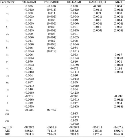
Table 2.2 reports the MLE estimates with standard errors in brackets, and
corresponding log likelihood values using threshold GARCH (1,1)-jump AR
(1) model (TS-GARJI), threshold GARCH (1,1) model (TS-GARCH),and regime
switching GARCH (1,1)-jump AR (1) model (RS-GARJI), together with the
re-sults using GARCH (1,1) model. Akaike’s information criterion and Bayesian
information criterion are also included to compare goodness of fit of models.
Table 2.2 shows that the parameters in the threshold GARJI model are
significant except the intercepts in the GARCH variance term and the jump
intensity AR (1) term. For the regime switching GARJI model, the
Table 2.2: Estimates and log likelihood values using different models
Parameter TS-GARJI TS-GARCH RS-GARJI GARCH(1,1) ARJI
µ 0.035 -0.006 0.038 -0.007 0.034 (0.012) (0.011) (0.012) (0.011) (0.012)
ω1 0.003 0.011 0.014 0.009 0.003 (0.002) (0.002) (0.004) (0.001) (0.001)
a1 0.011 0.033 0.019 0.041 0.014
(0.005) (0.005) (0.006) (0.004) (0.004)
b1 0.966 0.938 0.961 0.941 0.968
(0.013) (0.008) (0.013) (0.006) (0.008)
ω2 0.009 0.006 0.001
(0.006) (0.004) (0.002)
a2 0.011 0.062 0.008 (0.006) (0.008) (0.004)
b2 0.956 0.920 0.984 (0.024) (0.012) (0.031)
α1 0.006 0.063 0.017
(0.005) (0.104) (0.008)
ρ1 0.970 0.640 0.901
(0.024) (0.582) (0.048)
γ1 0.081 -0.077 0.184
(0.048) (0.111) (0.066)
α2 0.004 0.026
(0.003) (0.014)
ρ2 0.987 0.935
(0.011) (0.098)
γ2 0.146 0.964
(0.058) (0.423)
θ -0.219 -0.265 -0.292
(0.066) (0.071) (0.082)
δ 0.912 0.917 0.984
(0.075) (0.083) (0.088)
ν0 20.235 22.765
p11 0.983
(0.017)
p22 0.953
(0.053)
is the less volatile regime with a much smaller unconditional variance, it
im-plies that there are no jumps in the less volatile period. Therefore the regime
switching GARJI model is re-estimated with only jumps in the more volatile
period. Both AIC and BIC suggest that the threshold GARJI model has the
best fit of data among all the models, while GARCH (1,1) model has the worst.
The parameters in threshold GARJI model satisfy the stationarity condition,
and in each regime the summation ofaand b are less than one. The threshold
GARCH (1,1) model has a threshold value at 70%, which implies that there is
30% chance that the conditional variance shifts to regime 2. For the
thresh-old GARJI model, the threshthresh-old value is at 55%, implying that there is chance
of 45% for the conditional variance and jump intensity to shift to regime 2.
Including jump term better fits the data, as the threshold GARJI model
out-performs the threshold GARCH (1,1) model. Figure 2.1 and Figure 2.2 plot the
time series of the threshold variable, VIX, and the estimated threshold value
for the threshold GARCH model and the threshold GARJI model respectively,
showing that they have similar estimates in magnitude for the threshold value.
The mean reported in Table 2.2 for the threshold GARJI and the
regime-switching GARJI model are not the mean of the return, which is the reason
that it is different from the mean of return in the GARCH (1,1) model. The
mean of return is E(Rt) = µ+θE(λt) instead of µ for the jump models. The
persistence parameters in the jump intensity process are high for both regimes
that the persistence parameter in the diffusive conditional variance process is
lower in each regime than in the GARCH (1,1) model. However, after jumps
are incorporated, the persistence parameter in the conditional variance process
is higher in each regime for both the threshold GARJI model and the regime
switching GARJI model than in the GARCH (1,1) model. It implies that
sep-arating the effects of jumps and diffusive volatility makes the volatility more
persistent, while the high persistence of diffusive volatility of the GARCH (1,1)
model may come from the reason that different regimes are not identified.
2.5
Forecasting
When forecasting volatility it is difficult to know what to compare the forecasts
with, since volatility is unobserved. Consequently, we use realized volatility
as the proxy ex post daily volatility to measure the forecasting performance
of regime switching GARCH-Jump models. The data set for constructing the
realized volatility contains the five-minute transaction price for the Japanese
Yen-US dollar spot exchange rate from January 12th, 2004 to January 11th,
2005. I use five minute data as it is considered the highest frequency at which
prices are less distorted by the market microstructure noise. Following
An-dersen and Bollerslev (1998), the trading day t starts from 21:00 GMT on day
0 500 1000 1500 2000 2500 3000 3500 5
10 15 20 25 30 35 40 45 50
threshold
0 500 1000 1500 2000 2500 3000 3500 5
10 15 20 25 30 35 40 45 50
threshold
local time take place during this period. Weekend days and major holidays are
deducted for the reason of too many missing values or slower trading pattern.
251 days are left after the deduction.
The mth five-minute exchange rate on day t is denoted by Pm,t, for m =
1,2, ..., M. For five-minute data, M = 288. The five minute return rm,t is
con-structed as rm,t = 100(lnPm,t−lnPm−1,t), for m = 1,2, ..., M, andt = 1,2, ...,251.
The realized volatility is obtained by summing up the squared intra-day
5-minute returns asRVt = ∑M
m=1r2m,t. Andersen and Bollerslev (1998) note that,
under a jump-diffusion semi-martingale setting for the price process with bounded
jump intensityλt, the realized volatility is consistent for quadratic variation of
the logarithmic price process. As the quadratic variation consists of both the
diffusive volatility and the cumulative squared jumps, the realized volatility
is a good proxy for volatility when jumps are taken into consideration as in
our models. Figure 2.3 plots the evolution of the realized volatility constructed
using 5-minute intraday returns in the out-of-sample period.
The respective parameters estimated from in-sample period are used to
con-duct conditional variance forecasts for all the models. The threshold variable is
still chosen as VIX and the threshold value is taken as the in-sample estimate.
A rolling scheme is used, that is, the in-sample period contains 3500
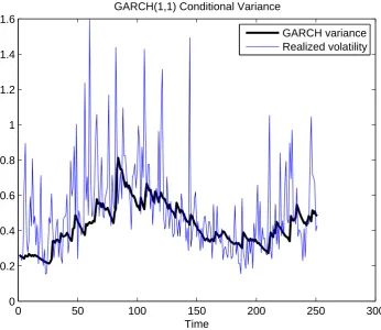
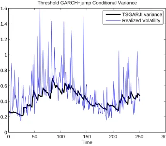
observa-tions and moves forward every 50 observaobserva-tions. Figure 2.4, Figure 2.5 and
Fig-ure 2.6 depict the out-of-sample one-step-ahead forecasts of conditional
respectively. From the figures we note that conditional variances conducted
from the Markov regime-switching GARCH-jump model has a bigger variation
than those from the GARCH(1,1) model and threshold GARCH-jump model.
Although the Markov regime-switching GARCH-jump model fits the data
bet-ter sometimes when there is a peak in the realized volatility, it also makes
some worse forecasts. When realized volatility is quite high, conditional
vari-ance from the threshold GARCH-jump model cannot catch up with it. One
possible reason is that jump size could be an increasing function of volatility.
AsV ar(Rt|Φt−1) =σt2+ (θ2+δ2)λt,θandδ can also play a role in determine the
conditional variance. They can be functions ofσtorλt.
For evaluating the forecasts, we run a linear regression of realized volatility
on its forecast. Then the coefficient of determination, R2, provides a guide to
the accuracy of volatility forecasts. The one-day-ahead out-of-sample volatility
forecasts are evaluated using the following regression,
RVt=c+dV ar(R(t)|Φt−1) +errort (2.40)
whereV art−1(R(t))is the out-of-sample conditional variance forecast for day t
of the corresponding model. R2 can be used to evaluate forecasting models as
it shows how much of the variation in realized volatility can be explained by
the variation of conditional variance forecasts. Table 2.3 reports the R2 for
0 50 100 150 200 250 300 0
0.2 0.4 0.6 0.8 1 1.2 1.4 1.6
Time Realized Volatility
Figure 2.3: Out-of-sample realized volatility from Jan 2004 to Jan 2005
Table 2.3: Out-of-sample evaluation statistics of conditional variance forecasts
TS-GARJI TS-GARCH RS-GARJI ARJI GARCH (1,1)
0 50 100 150 200 250 300 0
0.2 0.4 0.6 0.8 1 1.2 1.4 1.6
Time
GARCH(1,1) Conditional Variance
GARCH variance Realized volatility
0 50 100 150 200 250 300 0
0.2 0.4 0.6 0.8 1 1.2 1.4 1.6
Time
Threshold GARCH−jump Conditional Variance
TSGARJI variance Realized Volatility
0 50 100 150 200 250 300 0
0.2 0.4 0.6 0.8 1 1.2 1.4 1.6
Time
Markov Regime−switching GARCH−jump Conditional Variance
RSGARJI variance Realized Volatility
From the table we find that threshold GARJI model performs better to
ex-plain the variation of the data out-of-sample in terms of R2 than the
single-regime ARJI model. The reason is that the out-of-sample period is a tranquil
period, in which only one out of 251 observations has an absolute value that
is larger than 2; however, in the in-sample period, there are 58 out of 3500
observations whose absolute values are larger than 2. Thus the ARJI model
overestimates the jump part and leads to inaccurate forecasts. The threshold
GARJI model has the advantage of distinguishing the tranquil period from the
volatile period, leading to more accurate forecasting performance. Although
the single-regime ARJI model does not perform as well as the GARCH (1,1)
model, it does not imply that there is no need to incorporate jumps, as the
threshold GARJI model has a higher R2 than the GARCH (1,1) model. The
performance of the Markov regime-switching GARJI model is not good, which
is generally found in the exchange rate literature.
2.6
Conclusion
In this chapter we have developed two models to model jumps and regime
switching at the same time. The data generating process is assumed to be
a combination of a GARCH process capturing small and smooth changes and a
and abrupt changes in return. Therefore, the volatility process is affected by
both components. Meanwhile, we present switching regimes in the models to
account for the phenomenon that there are tranquil periods when jumps rarely
happen and volatile periods when jumps are more likely to happen. Regimes
are incorporated either using a hidden first-order Markov process or through
an exogenous threshold variable. For the Markov regime-switching GARJI
model, the jump intensity is assumed to depend on the expected lagged
in-tensity conditional on the current state, in order to solve the problem of regime
path dependence. In each regime, both the GARCH variance and the jump
intensity process have different parameter settings.
In the Markov regime-switching GARJI model, regimes are unknown to the
econometrician. As the one-day-ahead state of regime is unknown, it leads to
difficulty in forecasting. Therefore, a threshold GARCH-jump model is also
proposed. The one-day-ahead state of regime is known to the econometrician
by comparing the threshold variable and the threshold value. The stationarity
conditions and moments of returns are derived for the threshold GARCH-jump
model with an exogenous threshold variable. Both models are estimated using
maximum likelihood method, and the regime-switching GARCH-jump model
are more computationally intensive than the threshold GARCH-jump model.
realized volatility constructed from 5-minute intraday data as proxy of
volatil-ity for evaluation of forecasts of different models. The empirical results
indi-cate that jump intensity has a significant level of persistence, and the regime
switching GARCH-jump models outperform GARCH model for the in-sample
period. We also find that the persistence of diffusive volatility is lower for a
threshold GARCH (1,1) than a single regime GARCH model, which is in
accor-dance with previous literature. Out-of-sample forecasts suggest that threshold
GARCH-jump model has a good ability to forecast volatility of Japanese
Yen-US Dollar exchange rate and it outperforms the single regime ARJI model,
2.7
Bibliography
ANDERSEN, T., ANDT. BOLLERSLEV(1998): “Answering skeptics:Yes,standard
volatility models do provide accurate forecasts,”International Economic
Re-views, 39, 115–158.
BARNDOFF-NIELSEN, O.,ANDN. SHEPHARD(2001): “Non-Gaussian
Ornstein-Unlenbeck models and some of their uses in financial economics,”The Royal
Statistical Society, B63, 167–241.
BARNDOFF-NIELSEN, O., ANDN. SHEPHARD(2004): “Power and bipower
vari-ation with stochastic volatility and jumps,”Journal of Financial
Economet-rics, 2, 1–37.
CHAN, W., AND J. M. MAHEU (2002): “Conditional jump dynamics in stock market returns,”Journal of Business&Economic Statistics, 20(3), 377–389.
DAS, S., AND R. K. SUNDARAM (1997): “Taming the skew: Higher-order mo-ments in modelling asset price processes in finance, NBER Working Paper
5976,” .