Sparse Array Signal Processing: New Array Geometries, Parameter Estimation, and Theoretical Analysis

(1)

Sparse Array Signal Processing: New Array Geometries,

Parameter Estimation, and Theoretical Analysis

Thesis by Chun-Lin Liu

In Partial Fulfillment of the Requirements for the degree of

Doctor of Philosophy

CALIFORNIA INSTITUTE OF TECHNOLOGY Pasadena, California

2018

(2)

c

2018

Chun-Lin Liu

(3)

ACKNOWLEDGEMENTS

First of all, I would like to express my deepest gratitude to my advisor, Professor P. P. Vaidyanathan, for his advice, guidance, patience, and encouragements, during the years of my PhD study at Caltech. He is an incredibly inspiring scholar and an excellent teacher. His unique insights into fundamental problems have broad-ened my horizons of scientific research. He taught me to explore various research topics in array signal processing, to ask influential and fundamental questions, and to think differently and creatively. Another valuable skill I learned from him is to write papers and to make presentations. I am also very thankful for his generous support whenever I faced difficulties. I am so fortunate to be advised by Professor P. P. Vaidyanathan during my PhD.

I would like to thank the members of my defense and candidacy committees: fessor Yaser Abu-Mostafa, Professor Shuki Bruck, Professor Victoria Kostina, Pro-fessor Babak Hassibi, and ProPro-fessor Venkat Chandrasekaran. I learned a lot from their courses and valuable comments on my research.

Generous support from the Office of Naval Research (ONR), the National Science Foundation (NSF), California Institute of Technology, and Taiwan/Caltech Ministry of Education Fellowship is gratefully acknowledged.

I would like to thank the past and present members of my group, Professor See-May Phoong, Professor Yuan-Pei Lin, Professor Borching Su, Professor Piya Pal, Srikanth Tenneti, and Oguzhan Teke, for their generous support and valuable discussions. I would like to thank Caroline Murphy, Tanya Owen, and Carol Sosnowski for their administrative assistance. I am also very thankful to the colleagues working in sig-nal processing, communications, physics, and mathematics for their inspiring work. Many thanks to Kuan-Chang Chen, Yu-Hung Lai, Albert Chern, Lucas Peng, all my friends, and their associates in Association of Caltech Taiwanese for their company during my PhD. I am very thankful to Tui Tsai for his kind support, especially in my first year at Caltech. I would like to thank my friends in Taiwan, in the United States, and in Europe for their friendships.

(4)

with research ideas, to organize experimental results, to write papers, and to make slides as well as posters.

(5)

ABSTRACT

Array signal processing focuses on an array of sensors receiving the incoming wave-forms in the environment, from which source information, such as directions of ar-rival (DOA), signal power, amplitude, polarization, and velocity, can be estimated. This topic finds ubiquitous applications in radar, astronomy, tomography, imag-ing, and communications. In these applications, sparse arrays have recently at-tracted considerable attention, since they are capable of resolving O(N2) uncor-related source directions withN physical sensors. This is unlike the uniform linear arrays (ULA), which identify at mostN −1uncorrelated sources withN sensors. These sparse arrays include minimum redundancy arrays (MRA), nested arrays, and coprime arrays. All these arrays have an O(N2)-long central ULA segment in the difference coarray, which is defined as the set of differences between sensor locations. This O(N2) property makes it possible to resolveO(N2) uncorrelated sources, using onlyN physical sensors.

The main contribution of this thesis is to provide a new direction for array geometry and performance analysis of sparse arrays in the presence of nonidealities. The first part of this thesis focuses on designing novel array geometries that are robust to effects of mutual coupling. It is known that, mutual coupling between sensors has an adverse effect on the estimation of DOA. While there are methods to counteract this through appropriate modeling and calibration, they are usually computation-ally expensive, and sensitive to model mismatch. On the other hand, sparse arrays, such as MRA, nested arrays, and coprime arrays, have reduced mutual coupling compared to ULA, but all of these have their own disadvantages. This thesis intro-duces a new array called the super nested array, which has many of the good prop-erties of the nested array, and at the same time achieves reduced mutual coupling. Many theoretical properties are proved and simulations are included to demon-strate the superior performance of super nested arrays in the presence of mutual coupling.

Two-dimensional planar sparse arrays with large difference coarrays have also been known for a long time. These include billboard arrays, open box arrays (OBA), and 2D nested arrays. However, all of them have considerable mutual coupling. This thesis proposes new planar sparse arrays with the same large difference coarrays as the OBA, but with reduced mutual coupling. The new arrays include half open box arrays (HOBA), half open box arrays with two layers (HOBA-2), and hourglass ar-rays. Among these, simulations show that hourglass arrays have the best estimation performance in presence of mutual coupling.

(6)

the-oretical perspective. We first study the Cramér-Rao bound (CRB) for sparse arrays, which poses a lower bound on the variances of unbiased DOA estimators. While there exist landmark papers on the study of the CRB in the context of array pro-cessing, the closed-form expressions available in the literature are not applicable in the context of sparse arrays for which the number of identifiable sources exceeds the number of sensors. This thesis derives a new expression for the CRB to fill this gap. Based on the proposed CRB expression, it is possible to prove the previously known experimental observation that, when there are more sources than sensors, the CRB stagnates to a constant value as the SNR tends to infinity. It is also possible to precisely specify the relation between the number of sensors and the number of uncorrelated sources such that these sources could be resolved.

Recently, it has been shown that correlation subspaces, which reveal the structure of the covariance matrix, help to improve some existing DOA estimators. However, the bases, the dimension, and other theoretical properties of correlation subspaces remain to be investigated. This thesis proposes generalized correlation subspaces in one and multiple dimensions. This leads to new insights into correlation sub-spaces and DOA estimation with prior knowledge. First, it is shown that the bases and the dimension of correlation subspaces are fundamentally related to difference coarrays, which were previously found to be important in the study of sparse ar-rays. Furthermore, generalized correlation subspaces can handle certain forms of prior knowledge about source directions. These results allow one to derive a broad class of DOA estimators with improved performance.

It is empirically known that the coarray structure is susceptible to sensor failures, and the reliability of sparse arrays remains a significant but challenging topic for in-vestigation. This thesis advances a general theory for quantifying such robustness, by studying the effect of sensor failure on the difference coarray. We first present the (k-)essentialness property, which characterizes the combinations of the faulty sen-sors that shrink the difference coarray. Based on this, the notion of (k-)fragility is proposed to quantify the reliability of sparse arrays with faulty sensors, along with comprehensive studies of their properties. These novel concepts provide quite a few insights into the interplay between the array geometry and its robustness. For instance, for the same number of sensors, it can be proved that ULA is more robust than the coprime array, and the coprime array is more robust than the nested ar-ray. Rigorous development of these ideas leads to expressions for the probability of coarray failure, as a function of the probability of sensor failure.

(7)

PUBLISHED CONTENT AND CONTRIBUTIONS

[1] C.-L. Liu and P. P. Vaidyanathan, “Remarks on the spatial smoothing step in coarray MUSIC,”IEEE Signal Process. Lett., vol. 22, no. 9, pp. 1438–1442, Sep. 2015. doi:10.1109/LSP.2015.2409153,

The content of this paper is the preliminary version of Chapter 2.

[2] C.-L. Liu and P. P. Vaidyanathan, “Super nested arrays: Linear sparse ar-rays with reduced mutual coupling–Part I: Fundamentals,”IEEE Trans. Sig-nal Process., vol. 64, no. 15, pp. 3997–4012, Aug. 2016, issn: 1053-587X. doi:

10.1109/TSP.2016.2558159,

The content of this paper is described in Chapter 3.

[3] C.-L. Liu and P. P. Vaidyanathan, “Super nested arrays: Sparse arrays with less mutual coupling than nested arrays,” in Proc. IEEE Int. Conf. Acoust., Speech, and Sig. Proc., Shanghai, China, Mar. 2016, pp. 2976–2980. doi: 10 .

1109/ICASSP.2016.7472223,

[4] C.-L. Liu and P. P. Vaidyanathan, “Super nested arrays: Linear sparse arrays with reduced mutual coupling–Part II: High-order extensions,”IEEE Trans. Signal Process., vol. 64, no. 16, pp. 4203–4217, Aug. 2016, issn: 1053-587X. doi:

10.1109/TSP.2016.2558167,

[5] C.-L. Liu and P. P. Vaidyanathan, “High order super nested arrays,” inProc. IEEE Sensor Array and Multichannel Signal Process. Workshop, Jul. 2016, pp. 1– 5. doi:10.1109/SAM.2016.7569621,

[6] C.-L. Liu and P. P. Vaidyanathan, “Hourglass arrays and other novel 2-D sparse arrays with reduced mutual coupling,” IEEE Trans. Signal Process., vol. 65, no. 13, pp. 3369–3383, Jul. 2017, issn: 1053-587X. doi:10.1109/TSP.

2017.2690390,

[7] C.-L. Liu and P. P. Vaidyanathan, “Two-dimensional sparse arrays with hole-free coarray and reduced mutual coupling,” inProc. IEEE Asil. Conf. on Sig., Sys., and Comp., Nov. 2016, pp. 1508–1512. doi:10.1109/ACSSC.2016.7869629, The content of this paper is the preliminary version of Chapter 5.

[8] C.-L. Liu and P. P. Vaidyanathan, “Cramér-Rao bounds for coprime and other sparse arrays, which find more sources than sensors,”Digit. Signal Process., vol. 61, pp. 43–61, Feb. 2017, Special Issue on Coprime Sampling and Arrays, issn: 1051-2004. doi:10.1016/j.dsp.2016.04.011,

(8)

[10] C.-L. Liu and P. P. Vaidyanathan, “Correlation subspaces: Generalizations and connection to difference coarrays,”IEEE Trans. Signal Process., vol. 65, no. 19, pp. 5006–5020, Oct. 2017, issn: 1053-587X. doi:10.1109/TSP.2017.

2721915,

[11] C.-L. Liu and P. P. Vaidyanathan, “The role of difference coarrays in correla-tion subspaces,” inProc. IEEE Asil. Conf. on Sig., Sys., and Comp., Oct. 2017, pp. 1173–1177. doi:10.1109/ACSSC.2017.8335536,

[12] C.-L. Liu and P. P. Vaidyanathan, “Robustness of coarrays of sparse arrays to sensor failures,” inProc. IEEE Int. Conf. Acoust., Speech, and Sig. Proc., Apr. 2018,

[13] C.-L. Liu and P. P. Vaidyanathan, “Maximally economic sparse arrays and Cantor arrays,” in Proc. IEEE Int. Workshop on Comput. Advances in Multi-Sensor Adaptive Process., Dec. 2017, pp. 1–5. doi:10 . 1109 / CAMSAP . 2017 . 8313139,

Contributions

(9)

TABLE OF CONTENTS

Acknowledgements . . . iii

Abstract . . . v

Published Content and Contributions . . . vii

Table of Contents . . . ix

List of Illustrations . . . xii

List of Tables . . . xxi

Chapter I: Introduction . . . 1

1.1 Review of Array Equation . . . 2

1.2 The Role of Array Geometry in DOA Estimation . . . 6

1.3 Scope and Outline of the Thesis . . . 9

1.4 Notations . . . 13

Chapter II: Coarray MUSIC and Spatial Smoothing . . . 16

2.1 Introduction . . . 16

2.2 Review of Sparse Arrays . . . 17

2.3 Review of MUSIC and Spatial Smoothing MUSIC . . . 23

2.4 Coarray MUSIC without Spatial Smoothing . . . 29

2.5 Discussions . . . 31

2.6 Concluding Remarks . . . 35

Chapter III: Super Nested Arrays: Linear Sparse Arrays with Reduced Mutual Coupling: Fundamentals . . . 36

3.2 Review of Mutual Coupling . . . 39

3.3 Mutual Coupling in Sparse Arrays: A Motivating Example . . . 41

3.4 Second-Order Super Nested Arrays . . . 45

3.5 Coarray of Second-Order Super Nested Arrays . . . 49

3.6 Numerical Examples . . . 55

Chapter IV: High Order Super Nested Arrays . . . 65

4.2 General Guidelines for the Construction of Super Nested Arrays . . . 66

4.3 Qth-Order Super Nested Arrays,N1is Odd . . . 69

4.4 Qth-Order Super-Nested Arrays,N1is Even . . . 75

4.5 Proof of Theorem 4.3.1 . . . 80

4.6 Proof of Theorem 4.4.1 . . . 88

Chapter V: Hourglass Arrays, and Other Novel 2D Sparse Arrays with Re-duced Mutual Coupling . . . 99

5.2 Preliminaries . . . 101

(10)

5.4 Reorganization ofH1 andH2in OBA . . . 108

5.5 Half Open Box Arrays with Two Layers (HOBA-2) . . . 110

5.6 Hourglass Arrays . . . 112

5.7 Weight Functions . . . 115

5.A Proof of Lemma 5.3.1 . . . 125

5.B Proof of Lemma 5.3.2 . . . 125

5.C Proof of Theorem 5.3.1 . . . 126

5.D Proof of Theorem 5.4.1 . . . 128

5.E Proof of Theorem 5.6.1 . . . 131

Chapter VI: Cramér-Rao Bounds for Sparse Arrays, which Find More Source Directions than Sensors . . . 134

6.2 The Data Model and Sparse Arrays . . . 137

6.3 Review of Cramér-Rao Bounds . . . 139

6.4 New Expressions for CRB, Applicable for Sparse Arrays with More Sources than Sensors . . . 143

6.5 Conclusions which Follow from Theorem 6.4.2 . . . 149

6.6 Connection to the ULA Part of the Coarray . . . 152

6.A Derivation to the Proposed CRB Expression . . . 162

6.B Definition ofJ . . . 165

6.C Proof of the Asymptotic CRB Expression for Large SNR . . . 167

6.D Proof of Theorem 6.6.1 . . . 170

Chapter VII: Correlation Subspaces: Generalizations and Connection to Dif-ference Coarrays . . . 173

7.2 Review of Correlation Subspaces . . . 174

7.3 Generalized Correlation Subspaces . . . 178

7.4 Properties of Generalized Correlation Subspaces . . . 179

7.5 Connections with Existing Methods . . . 190

7.6 Generalized Correlation Subspaces in Multiple Dimensions . . . 193

7.A Proof of the Equivalence of (7.5) and Definition 7.2.1 . . . 201

7.B Proof of Lemma 7.3.1 . . . 202

7.C Properties of Weight Functions . . . 202

7.D Numerical Examples for Section 7.6 . . . 204

7.E Derivation of (7.63) . . . 206

Chapter VIII: Robustness of Difference Coarrays of Sparse Arrays to Sensor Failures – A General Theory . . . 209

8.2 The Essentialness Property . . . 211

8.3 Thek-Fragility . . . 223

8.4 Thek-Essential Sperner Family . . . 225

(11)

Chapter IX: Robustness of Difference Coarrays of Sparse Arrays to Sensor Fail-ures – Array Geometries . . . 238

9.2 Maximally Economic Sparse Arrays . . . 239

9.3 Uniform Linear Arrays . . . 247

9.4 Coprime Arrays . . . 253

Chapter X: Conclusions and Future Directions . . . 267

(12)

LIST OF ILLUSTRATIONS

Number Page

1.1 A basic model for array signal processing. . . 3 1.2 Conversion from the physical sensor locations to the normalized

sen-sor locations. . . 4 1.3 DOA estimation using uniform linear arrays (left) and sparse arrays

(right). Here red dots denote physical sensors and crosses represent empty space. . . 7 1.4 The physical arrays (a)S1, (c)S2, (e)S3, and their difference coarrays

(b) D1, (d) D2, (f)D3. In these figures, dots denote elements in a set while crosses represent the empty space. . . 8 2.1 An illustration of the setsS, D, U,V, and the weight functionw(m).

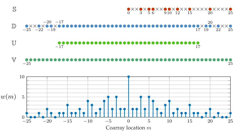
Here we consider a coprime array withM = 3andN = 5, as defined in (2.8). . . 19 2.2 The array geometriesS, the difference coarraysD, and the weight

func-tionsw(m)of (a) the MRA with6sensors, (b) the MHA with6sensors, (c) the nested array withN1=N2= 3, and (d) the coprime array with M = 2, N = 3. All these arrays have6physical sensors. InSandD, dots denote elements and crosses represent empty locations. . . 20 2.3 A schematic diagram of the MUSIC algorithm. . . 24 2.4 The conversion from theReS_{to the autocorrelation vector}_exD_. _{. . . . .} ₂₈ 2.5 The MUSIC spectrum based on anM = 5, N = 7coprime array,0dB

SNR,K = 500snapshots, and the Hermitian Toeplitz matrixRe. D= 35sources are placed uniformly overθ¯∈[−0.49,0.49]. The number of sensors isN+ 2M−1 = 16. . . 34 3.1 The concept of 2D representations of linear arrays. The top of this

(13)

3.2 The 1D and 2D representations of a second-order super nested array withN1 =N2= 5. It will be proved in this chapter that super nested arrays possess the same number of sensors, the same physical aper-ture, and the same hole-free coarray as their parent nested arrays. Fur-thermore, super nested arrays alleviate the mutual coupling effect. In this example, there is only one pair of sensors with separation 1, lo-cated at 29and30. However, for the parent nested array in Fig. 3.1, locations1through6are crowded with sensors, leading to more se-vere mutual coupling effect. . . 37 3.3 Comparison among ULAs, MRAs, nested arrays, coprime arrays and

their MUSIC spectraP(¯θ)in the presence of mutual coupling. It can be observed that higher uniform DOF and smaller weight functions w(1),w(2),w(3)tend to decrease the RMSE. . . 42 3.4 1D representations of second-order super nested arrays with (a)N1 =

10, N2 = 4, and (b)N1 = N2 = 7. Bullets stand for physical sensors and crosses represent empty space. Both configurations consist of14 physical sensors but (b) leads to larger total aperture and a sparser pattern. It will be proved that the uniform DOF of (a) and (b) are 2N2(N1+ 1)−1, which are87and111, respectively. . . 45 3.5 2D representations of (a) the parent nested array, and (b) the

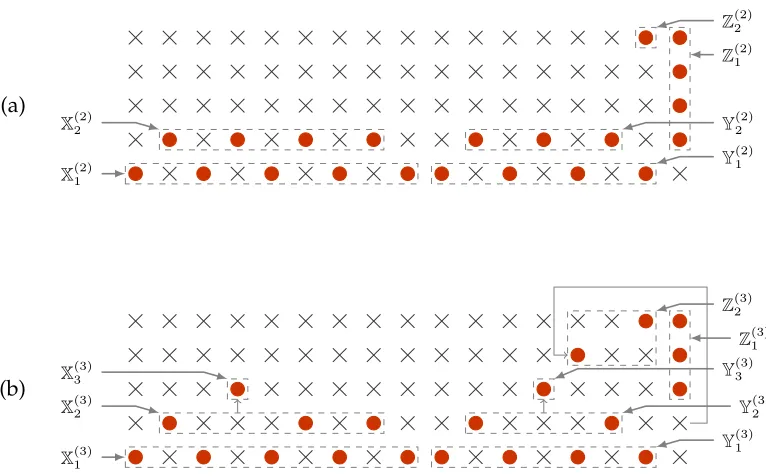
corre-sponding second-order super nested array, S(2), where N1 = N2 = 13. Bullets denote sensor locations while crosses indicate empty loca-tions. Thin arrows illustrate how sensors migrate from nested arrays to second-order super nested arrays. The dense ULA in nested arrays is split into four sets: X(2)1 ,Y

(2) 1 ,X

(2)

2 , andY (2)

2 in second-order super nested arrays. The sensor located atN1 + 1, belonging to the sparse ULA of nested arrays, is moved to locationN2(N1+ 1)−1in second-order super nested arrays. . . 47 3.6 Comparison among ULA, nested array, coprime array, second-order

super nested array, and third-order super nested array in the presence

of mutual coupling. The coupling leakageLis defined askC−diag(C)kF/kCkF,

(14)

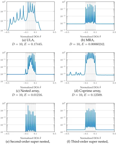
3.7 The MUSIC spectra P(¯θ) for ULA, MRA, nested arrays, coprime ar-rays, second-order super nested arar-rays, and third-order super nested arrays whenD = 10sources are located atθ¯i =−0.1 + 0.2(i−1)/9, i = 1,2, . . . ,10, as depicted by ticks and vertical lines. The SNR is0 dB while the number of snapshots is K = 500. Note that the num-ber of sources 10is less than the number of sensors 14. The mutual coupling is based on (3.3) with c1 = 0.3 exp (π/3), B = 100, and c`=c1exp (−(`−1)π/8)/`for2≤`≤B. . . 59 3.8 The MUSIC spectraP(¯θ)for MRA, nested arrays, coprime arrays,

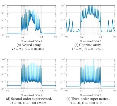
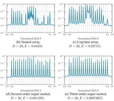
second-order super nested arrays, and third-second-order super nested arrays when D= 20sources are located atθ¯i=−0.2+0.4(i−1)/19,i= 1,2, . . . ,20, as depicted by ticks and vertical lines. The SNR is0dB while the num-ber of snapshots isK = 500. Note that the number of sources20 is greater than the number of sensors14. The mutual coupling is based on (3.3) withc1 = 0.3 exp (π/3),B = 100, andc` =c1exp (−(`−1)π/8)/` for2≤`≤B. . . 60 3.9 The MUSIC spectraP(¯θ)for MRA, nested arrays, coprime arrays,

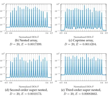
second-order super nested arrays, and third-second-order super nested arrays when D= 20sources are located atθ¯i =−0.4+0.8(i−1)/19,i= 1,2, . . . ,20, as depicted by ticks and vertical lines. The SNR is0dB while the num-ber of snapshots is K = 500. The mutual coupling is based on (3.3) withc1 = 0.3 exp (π/3),B = 100, andc` = c1exp (−(`−1)π/8)/` for2≤`≤B. . . 62 3.10 Based on the practical mutual coupling model (3.2), the MUSIC

spec-tra P(¯θ) are listed for MRA, nested arrays, coprime arrays, second-order super nested arrays, and third-second-order super nested arrays, where D= 20sources are located atθ¯i =−0.4+0.8(i−1)/19,i= 1,2, . . . ,20. The SNR is0dB while the number of snapshots isK = 500. The pa-rameters in (3.2) are given byZA=ZL= 50ohms andl=λ/2. . . 64 4.1 Hierarchy of nested arrays, second-order super nested arraysS(2), and

Qth-order super nested arraysS(Q). Arrows indicate the origin of the given sets. For instance, X(4)2 originates from X

(3)

2 whileY (3)

3 is split intoY(4)3 andY

(4)

4 . It can be observed that the setsX (Q)

q andY(qQ)result from the dense ULA part of nested arrays. The sparse ULA portion of nested arrays is rearranged into the setsZ(1Q)andZ

(Q)

2 . . . 67 4.2 1D representations of (a) second-order super nested arrays,S(2), and

(15)

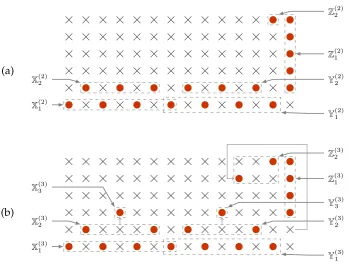
4.3 2D representations of (a) second-order super nested arrays,S(2), and (b) third-order super nested arrays,S(3), whereN1 = 13andN2 = 6. Bullets denote sensor locations while crosses indicate empty locations. The dashed rectangles mark the sets X(qQ), Yq(Q), Z(1Q), and Z

(Q) 2 for 1≤q ≤Q. Thin arrows illustrate how sensors migrate fromS(Q−1)to

S(Q)

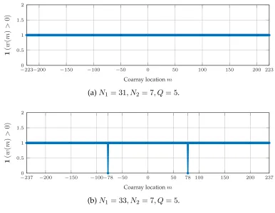
. . . 69 4.4 An example to show that N1 ≥ 3·2Q−1 is not necessary in order

to make the coarray ofS(Q)hole free. Here we consider the indicator function ofw(m)>0for the super nested array with (a)N1 = 31, N2 = 7, Q= 5and (b)N1 = 33, N2 = 7, Q= 5. It can be inferred that (a) is a restricted array, becausew(m) >0for−223≤ m ≤223. However, (b) is not a restricted array sincew(78) =w(−78) = 0. . . 73 4.5 2D representations of (a) the second-order super nested arrayS(2)and

(b) the third-order super nested arrayS(3), whereN1 = 16(even) and N2= 5. Bullets represent physical sensors while crosses denote empty space. Thin arrows illustrate the recursive rules (Rule 2 and Rule 3) in Fig. 4.1. . . 76 4.6 Estimation error as a function of source spacing∆¯θbetween two sources.

The parameters are SNR = 0dB, K = 500. The sources have equal power and their normalized DOA areθ¯1 = ¯θ0+ ∆¯θ/2andθ¯2 = ¯θ0 − ∆¯θ/2, whereθ¯0= 0.2. Each point is an average over1000runs. . . 94 4.7 Estimation error as a function of (a) SNR, (b) the number of snapshots

K, and (c) the number of sources D. The parameters are (a) K = 500, D = 20, (b)SNR = 0dB, D = 20, and (c)SNR = 0dB, K = 500. The sources have equal power and normalized DOA θ¯i = −0.45 +

0.9(i₋1)/(D₋1)for1 ≤i≤D. Each point is an average over1000 runs. . . 96 4.8 Estimation error as a function of mutual coupling coefficient c1 (see

Eq. (3.3)). The parameters areSNR = 0dB, K = 500, and the number of sources (a)D= 10, (b)D = 20, and (c)D= 40. The sources have equal power and are located atθ¯i = −0.45 + 0.9(i−1)/(D−1)for 1 _≤ i _≤ D. The mutual coupling coefficients satisfy|c`/ck| = k/`

while the phases are randomly chosen from their domain. Each point is an average over1000runs. . . 97 5.1 The array geometry of (a) open box arrays (OBA) and (b) hourglass

(16)

5.2 Examples of 2D arrays withN = 36elements. Bullets denote physical sensors and crosses represent empty space. The minimum separation between sensors isλ/2. . . 103 5.3 Examples of POBA withNx = 16andNy = 11. (a)g1 ={1,2,3,5,6,7,9,13},g2=

{1,3,4,5,7,11}, and (b)g1 =g2 ={1,3,5,7,9,11,13}. In both cases,

g₂_{satisfies Theorem 5.3.1.} _{. . . 106}

5.4 Examples of POBA-L.Nx = 16,Ny = 11,g1=g2={1,3,5,7,9,11,13}. (a) h1,1 = {1,3,5,7,9}, h1,2 = {2,4,6,8}, L = 2, and (b) h1,1 =

{1,2,4,6,8,9_},h1,2={3,7},h1,3 ={5},L= 3. . . 108 5.5 Examples of HOBA-2. (a)Nx = 16, Ny = 11and (b)Nx= 16, Ny = 12. 111 5.6 Hourglass arrays with (a)Nx = 15, Ny = 27and (b)Nx= 15, Ny = 26.

The total number of sensors for (a) and (b) are67and65, respectively. 114 5.7 The normalized source directions, as shown in circles, for the

exam-ples in Section 5.8. Here the number of sources Dis assumed to be a perfect square, i.e.,√Dis an integer. The sources are uniformly lo-cated in the shaded region, over which there are√Dequally-spaced sources in one way and

√

Dequally-spaced sources in the other. . . . 121 5.8 The RMSE as a function of (a) SNR and (b) the number of snapshots

K.The number of sensors is 81 for all arrays. The parameters are (a) K = 200_{, the number of sources}D = 9_{and (b)} 0_{dB SNR,} D = 9. The sources directions are depicted in Fig. 5.7. Each point is averaged from1000runs. . . 123 5.9 The RMSE as a function of the mutual coupling model for (a) the

num-ber of sourcesD= 9and (b)D= 36.The number of sensors is 81 for all arrays. The parameters are0dB SNR andK = 200. The sources di-rections are depicted in Fig. 5.7. The mutual coupling model is char-acterized byB = 5andc(`) = c(1) exp [π(`−1)/4]/`.Each point is averaged from1000runs. . . 124 6.1 The dependence of the proposed CRB expression on snapshots for

various numbers of sourcesD. The array configuration is the nested array withN1 =N2= 2so that the sensor locations areS={1,2,3,6}. The equal-power sources are located atθ¯i =−0.49 + 0.9(i−1)/Dfor i= 1,2, . . . , D. SNR is20dB. . . 153 6.2 The dependence of the proposed CRB expression on SNR for (a)D <

(17)

6.3 The dependence of the proposed CRB on (a) snapshots and (b) SNR for ULA, MRA, nested arrays, coprime arrays, and super nested ar-rays. The total number of sensors is 10and the sensor locations are given in (6.56) to (6.59). The number of sources isD= 3(fewer sources than sensors) and the sources are located atθ¯i =−0.49 + 0.99(i−1)/D

fori= 1,2, . . . , D. For (a), the SNR is20dB while for (b) the number of snapshotsKis500. . . 156 6.4 The dependence of the proposed CRB on (a) snapshots and (b) SNR

for MRA, nested arrays, coprime arrays, and super nested arrays. The total number of sensors is 10 and the sensor locations are given in (6.56) to (6.59). The number of sources isD= 17(more sources than sensors) and the sources are located atθ¯i =−0.49 + 0.99(i−1)/Dfor i = 1,2, . . . , D. For (a), the SNR is20dB while for (b) the number of snapshotsK is500. . . 157 6.5 The dependence of the proposed CRB on the number of sourcesDfor

various array configurations. The equal-power sources are located at ¯

θi =−0.49+0.99(i−1)/Dfori= 1,2, . . . , D. The number of snapshots K is500and SNR is20dB. . . 159 6.6 The CRB expressions versus the number of sourcesDfor a coprime

array. (a) The stochastic CRB expression [167], (b) the CRB which is evaluated numerically by Abramovich et al. [1], (c) Jansson et al.’s CRB expression [66], and (d) the proposed CRB expression, as in Theorem 6.4.2. The coprime array withM = 3,N = 5has sensor locations as in (6.59) and the difference coarray as in (6.64). The number of sensors

|S|= 10. The equal-power sources are located atθ¯i =−0.48+(i−1)/D

fori= 1,2, . . . , D. The number of snapshotsKis500and SNR is20 dB. . . 160 7.1 The density function in (7.16) (red), and the constant density function

in Section 7.4 (blue). . . 178 7.2 The sensor locationsSand the nonnegative part of the difference

coar-raysD+for (a) ULA with 10 sensors, (b) the nested array withN1 = N2 = 5, (c) the coprime array withM = 3, N = 5, and (d) the super nested array withN1 =N2 = 5, Q = 2. Here bullets denote elements inSorD+while crosses represent empty space. . . 185 7.3 (a) The eigenvalues and (b) the first four eigenvectors of the

general-ized correlation subspace matrixS(1[−α/2,α/2])in Example 7.4.3. Here the difference coarrayD={−29, . . . ,29}andαis0.1. . . 186 7.4 The dependence of the relative errorE(`)on the parameter`, where

(18)

7.5 The geometric interpretation of sample covariance matrix denoising using generalized correlation subspaces (Problem (P2)). The sample covariance matrix is denoted byReS. The vectorsp?₁andp?₂are the or-thogonal projections ofvec(ReS)ontoCS+Iand onto a subspace that approximatesGCS(1[−α/2,α/2])+I, respectively. HereI= span(vec(I)) and the sum between subspacesAandBis defined asA+B={a+b: a_{∈ A}, b_{∈ B}}. . . 190 7.6 The visible region (shaded) of (a) angle-Doppler, (b) 2D DOA, (c) 2D

DOA withθmin≤θ≤θmax, and (d) 2D DOA withφmin≤φ≤φmax. . 194 7.7 The eigenvalues of the matrix S(ρ)e _{(left) and the weight functions}

(right) for (a), (b) the ULA with 10 sensors (|D| = 19), (c), (d) the nested array with N1 = N2 = 5 (10 sensors, |D| = 59), (e), (f) the coprime array with M = 3, N = 5(10 sensors, |D| = 43), and (g), (h) the super nested array with N1 = N2 = 5, Q = 2 (10 sensors,

|D|= 59). Here the matricesS(ρ)e are given by (7.64) and the eigenval-ues ofS(ρ)e _{are obtained numerically. The red dashed curves in Figs.} (a), (c), (e), and (g) correspond toρ1(¯θ) = 2(1−(2¯θ)2)−1/21[−1/2,1/2](¯θ) while the blue curves in Figs. (a), (c), (e), and (g) are associated with ρ2(¯θ) =1[−1/2,1/2](¯θ). . . 197 7.8 The dependence of root mean-squared errors (RMSE) on (a) SNR and

(b) the number of snapshots for the optimization problems (P1) and (P2) with generalized correlation subspacesGCS(1[−α/2,α/2]). There areD= 3equal-power and uncorrelated sources at normalized DOAs

−0.045,0, and0.045. The array configuration is the nested array with N1 = N2 = 5(10 sensors), as depicted in Fig. 7.2(b). The parameters are (a) 100 snapshots and (b) 0dB SNR. Each data point is averaged from 1000 Monte-Carlo runs. . . 199 7.9 (a) The physical array and (b) its difference coarray. . . 204 7.10 Plots for the sinc functionsinc(x)and the jinc functionjinc(x). . . 207

(19)

8.2 An example of MESA. (a) The original array and its difference coarray. The array configurations and the difference coarrays after the deletion of (b) the sensor at0, (c) the sensor at1, (d) the sensor at4, or (e) the sensor at6, from the original array in (a). Here the sensors are denoted by dots while crosses denote empty space. . . 213 8.3 Array configurations and the difference coarrays for (a) the ULA with

9sensors, and the arrays after the removal of (b)1, (c)2, (d)7, (e){1,2}, and (f){1,7}from (a). . . 214 8.4 The ULA with6physical sensors, where the essential sensors and the

inessential sensors are denoted by diamonds and rectangles, respec-tively. Thek-essential subarrays are also listed. . . 216 8.5 The array geometries and the weight functions for (a) the ULA with6

sensors, (b) the MRA with6sensors, and (c) the MHA with6sensors. The sensors are depicted in dots while the empty space is shown in crosses. The definition ofMqin Theorem 8.2.1.3 leads toM1= 2, M2 = 2for (a),M1= 22, M2 = 4for (b), andM1= 30, M2 = 0for (c). . . 217 8.6 An illustration for the main idea of the proof of Theorem 8.2.1.1. Here

the array is the ULA with6sensors and thek-essential familyE1 and

E2are depicted in Fig. 8.4. . . 221 8.7 The directed graph G in the proof of (8.15), for (a) the ULA with 6

sensors, (b) the MRA with6sensors, and (c) the MHA with6sensors. The number of directed edges is (a) M1 = 2, (b) M1 = 22, and (c) M1 = 30. . . 223 8.8 The array geometries (top) and thek-fragilityFk(bottom) for (a) the

ULA with16sensors, (b) the nested array withN1 =N2 = 8, and (c) the coprime array withM = 4andN = 9. . . 225 8.9 An example of the underlying structure ofk-essential familyEk. Here

the ULA with 7 sensors, S = {0,1, . . . ,6}, is considered while the numbers in each small box denote a subarray. For instance, “0,1,2” represents the subarray{0,1,2}. . . 226 8.10 The relation betweenEk = SkandEk0 =∅. Here solid arrows

repre-sent logical implication while arrows with red crosses mean that one condition does not necessarily imply the other. . . 230 8.11 The probability that the difference coarray changes Pc and its lower

(20)

8.12 The dependence of the probability that the difference coarray changes Pcon the probability of single sensor failurepfor (a) the ULA with12 sensors, (b) the nested array withN1 = N2 = 6, and (c) the coprime array withM = 4andN = 5. Here the essential sensors (diamonds) and the inessential sensors (squares) are depicted on the top of this figure. Experimental data points (Exp.) are averaged from107 Monte-Carlo runs. The approximations ofPcare valid forp 1/12 due to (8.36). . . 236 9.1 The array geometry (S, in diamonds) and the nonnegative part of the

weight function (w(m), in dots) for (a) the MRA with8elements, (b) the MHA with 8elements, (c) the nested array with N1 = N2 = 4 (8elements), and (d) the Cantor array with8elements. Here crosses denote empty space. . . 241 9.2 The ULA with N = 10elements and thek-essential Sperner family

E0

1,E20, andE30. . . 248 9.3 (a) The ULA with10physical elementsSULAand its difference coarray.

The physical array (left) and the difference coarray (right) after remov-ing (b){7,8,9}, (c){1,2,8}, and (d){3,5,8}, fromSULA, respectively. Here bullets denote elements and crosses represent empty space. It can be observed that the difference coarrays of (b), (c), and (d) contain

{0,_±1, . . . ,_±6_}. . . 251 9.4 An illustration for thek-essential Sperner family of the coprime arrays

with (a)M = 4, N = 5and (b)M = 5, N = 4. In these figures, the coprime arrays are split into two sparse ULAs for clarity. . . 254 9.5 (a) the coprime arrayScoprimewithM = 7, N = 8and the nonnegative

part of the difference coarrayD. (b) The arrayS, where the elements in A = {16,32,56}are removed from Scoprime, and the nonnegative part of its difference coarrayD. . . 259 9.6 The array configurations for (a) ULA with10elements, (b) the coprime

array withM = 3, N = 5, (c) the nested array withN1=N2 = 5, and (d) the MRA with10elements. . . 264 9.7 The dependence of RMSE on the element failurepwith respect to the

(21)

LIST OF TABLES

Number Page

2.1 Some terminologies related to sparse arrays . . . 21

3.1 Ranges ofP1andP2 . . . 51

3.2 Ranges ofX(2)1 ∪(X (2) 1 + 1)andY (2) 1 ∪(Y (2) 1 + 1) . . . 52

4.1 27 cases in the proof of Theorem 4.3.1 . . . 81

4.2 Array profiles for the example in Section 4.7 . . . 93

5.1 Summary on the weight functions . . . 116

5.2 Sensor pairs forw(1,1)with oddNx . . . 119

6.1 Summary of several related CRB expressions for DOA estimation . . 142

6.2 Identifiable/non-identifiable regions for coarray MUSIC. . . 158

7.1 Generalized correlation subspaces with known source intervals . . . 184

(22)

C h a p t e r 1

INTRODUCTION

The heart of modern technology is the widespread use of sensors, which produce sensor outputs to sense the surroundings. Studying these outputs finds enormous and potential applications incommunications(5G, massive MIMO systems, mmWave communications) [6], [80], [143],biomedical engineering (medical imaging, bioinfor-matics, wearable technology) [170],remote sensing(satellite navigation, environmen-tal sensing) [43], and so forth. Among all these applications, manipulating these data under limited physical resources such as bandwidth, power, and the number of sensors is a major challenge even today. Recently, due to inexpensive compu-tation, this challenge has been addressed in the framework of sparse sensing. The key idea of sparse sensing is that, by exploitingprior knowledgeabout signals, only a small portion of high-dimensional big data is delivered tosignal processing algo-rithms to recover the low-dimensional information of interest. This paradigm makes it possible to achieve the above-mentioned applications with limited physical re-sources.

(23)

This thesis aims at answering the above fundamental and insightful questions, in the context of source localization in array signal processing, since it plays a cen-tral role in communication, radar, medical imaging, and radio astronomy [22], [82], [157], [170], [188]. Here sparse sampling is equivalent tosparse sensor array config-urationwhile the information inference corresponds to the estimation of direction-of-arrival (DOA), signal power, amplitude, polarization, and velocity of the sources.

Furthermore, the estimation performance can be analyzed and explained through the Cramér-Rao bounds,the generalized correlation subspace, andthe essentialness prop-erty. The main contributions of this thesis can be summarized as follows:

1. Sparse sampling(sparse array design): We proposed several one-dimensional and two-dimensional sparse array configurations that take advantage of the statistics of the source profile and the interference among sensors (mutual coupling) [89], [92]–[95], [98]. For the proposed arrays, it is possible to resolve more uncorrelated sources than sensorswith improved resolution, in the presence of mutual coupling.

2. Information inference(Parameter estimation with sparse arrays): We developed new and practical algorithms that estimate more uncorrelated sources than sensors from the sparse array [86]–[88], [104].

3. Theoretical analysis(Cramér-Rao bounds, generalized correlation subspace, and robustness analysis): Here we studied the expressions ofthe Cramér-Rao bounds for sparse arrays, which are theoretical limits for the estimation performance of unbiased estimators [91], [97]. The proposed expressions explain why more uncorrelated sources than sensors can be identified using sparse arrays. We also show that DOA estimators can be explained through the theory of the generalized correlation subspace, which further provides insights to the optimal estimators [96], [102]. Furthermore, we also propose a general theory of ana-lyzing the robustness of the difference coarray with respect to sensor failures [103].

The chapter outline is as follows. Section 1.1 reviews the data model commonly used in array signal processing. Section 1.2 discusses the interplay between array geometry and DOA estimation. Section 1.3 gives the outline and the scope of this thesis while Section 1.4 defines the notation used in this thesis.

1.1 Review of Array Equation

(24)

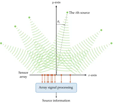
Array signal processing

Source information Sensor

array x-axis

y-axis

θi

[image:24.612.117.494.72.417.2]

Theith source

Figure 1.1: A basic model for array signal processing.

and assumptions in (1.5) will be explained comprehensively in the following devel-opment.

(25)

x-axis n-axis

0d

0 1d

1

8d

8

12d

12

14d

14

17d

17

d

S={0,1,8,12,14,17}

Figure 1.2: Conversion from the physical sensor locations to the normalized sensor locations.

source resides in the first quadrant, namely, thex-coordinate and they-coordinate are both positive, thenθi >0. By definition, the DOA of theith source satisfies

−π

2 ≤θi ≤ π

2. (1.1)

We begin by deriving the expressions for the sensor output signals induced by the sources. It is first assumed that all the sources aremonochromaticand all the prop-agating waves share the same frequencyf, hence the same wavelengthλ. Further-more, each source is concentrated at apointin thefar-fieldregion [188]. Therefore, the distances between the sources and the sensors are sufficiently large so that the wavefronts can be approximated byplane waves. It is also assumed that the propa-gating medium is homogeneous and lossless [68].

Next let us assume that the sensor locations belong to a uniform grid of step sized on thex-axis. Namely, the sensor locations can be specified bynd, wherenbelongs to an integer set S. The indices n are called normalized sensor locations, which are represented by an integer setS. In this thesis, unless stated separately, the nor-malized sensor locations, indicated by the setS, are used to characterize the array geometry. As an example, Fig. 1.2 demonstrates the conversion from the sensor lo-cations defined on thex-axis to those defined on the integer setS. Here the sensors are depicted in red solid circles and the empty space is illustrated using crosses. The physical sensors are located at0d,1d,8d,12d,14d, and17don thex-axis. After normalizing byd, we obtain the normalized sensor locationsS={0,1,8,12,14,17}. Based on the above-mentioned assumptions, the signal received by the sensor atnd can be expressed as [68], [188]

D

X

i=1 Aiexp

2πθ¯in

+w(n), (1.2)

where  , √−1, w(n) is the noise term, Ai is the complex amplitude of the ith source, andθ¯iis the normalized DOA of theith source, defined as

¯ θi ,

dsinθi

(26)

The model in (1.2) can be regarded as a linear combination of complex exponentials. Furthermore, the indexncan be regarded asspatial sample pointwhile the normal-ized DOAθ¯ican be interpreted asspatial frequency. Based on this interpretation, the step sizedcannot exceedλ/2, otherwise spatial ambiguity arises. Here spatial am-biguity is analogous to aliasing in the sampling theorem [68], [188]. In particular, if d > λ/2, then there exist multiple DOAs corresponding to the same array output, so that these DOAs become indistinguishable from the array output. Due to these, in this thesis, the step sizedis set to be

d= λ

2. (1.4)

Finally, Eq. (1.2) can be expressed as the following vector model: x_S=

D

X

i=1

AivS(¯θi) +nS, (1.5)

where the column vectorxS ∈ C|S|denotes the output of the overall sensor array andnSis the additive noise term. The steering vectorvS(¯θi)is defined asvS(¯θi) =

exp 2πθ¯in

n∈_S. In this thesis, the entries inxS,vS(¯θi), andnSare sorted in the

ascending order ofn ∈ S. That is, the first entry of xS corresponds to output of the leftmost sensor in the array while the last entry of xS is associated with the rightmost sensor.

Example 1.1.1. Let us consider the array geometry in Fig. 1.2. Due to (1.5), the column vectorsxS,vS(¯θi), andnScan be expressed as

          

Output atn= 0 Output atn= 1 Output atn= 8 Output atn= 12 Output atn= 14 Output atn= 17           

| {z }

x_S = D X i=1 Ai           

exp2πθ¯i·0

exp

2πθ¯i·1

exp2πθ¯i·8

exp2πθ¯i·12

exp

2πθ¯i·14

exp2πθ¯i·17

           | {z }

v_S(¯θi)

+           

Noise atn= 0 Noise atn= 1 Noise atn= 8 Noise atn= 12 Noise atn= 14 Noise atn= 17           

| {z }

n_S

. (1.6)

In practice, the array output (1.5) is repeatedK times, denoted byxS(k) fork = 1,2, . . . , K, to reduce the variation of the estimates. These vectorsxS(k)are called snapshotsof (1.5). In particular,xS(k)can be modeled as

x_S(k) =

D

X

i=1

Ai(k)vS(¯θi) +nS(k), k= 1,2, . . . , K. (1.7)

(27)

is to infer the information of interest, such as the DOA, source power, and so forth, based on the snapshots xS(k). More discussions on the snapshot model can be found in Chapter 2, Chapter 6, [188, Chapter 5], [68, Section 4.9], and the references therein.

As a remark, (1.5) assumes that the sources reside in the first and the second quad-rant of thexy-plane and the sensors are located on thex-axis. This scenario will be considered in most of the chapters, except for Chapter 5. Chapter 5 is based on two-dimensional array processing, where the sources are in the first four octants (z >0) in the three-dimensional space and the sensors are restricted to thexy-plane. In this case, the DOA of the source has two parameters: azimuth and elevation. All these details will be discussed in Chapter 5.

1.2 The Role of Array Geometry in DOA Estimation

Based on the array equation in (1.5),DOA estimation has been a popular research field in array processing for many decades and has found ubiquitous applications in radio astronomy, radar, imaging, communications, and so forth [22], [58], [68], [77], [157], [165], [188]. In particular, DOA estimation aims to infer the source directions, i.e.,θi fori = 1,2, . . . , D, from the array outputxS. This task can be divided into two stages:

Stage 1 Array geometry: According to the prior knowledge of the received signal, the goal here is to design an array geometryS(or sensor placement) that captures the information of interest efficiently.

Stage 2 Estimation: Given the array geometryS, this stage developsDOA estimators that infer the DOAs{θ1, θ2, . . . , θD}based on the array outputxS.

Uniform Linear Arrays (ULA)

(28)

λ Ai

θi

DOA Estimators Estimatedθi

λ/2

λ Ai

θi

Coarray-based DOA Estimators Estimatedθi

Difference coarray

λ/2

Figure 1.3: DOA estimation using uniform linear arrays (left) and sparse arrays (right). Here red dots denote physical sensors and crosses represent empty space.

Methods Of DOA Estimation (MODE) [162], and SParse Iterative Covariance-based Estimation (SPICE) [161],to name a few, have been developed for this purpose.

Sparse Arrays

It is known that ULA can resolve at mostN −1sources withN physical sensors, regardless of the choice of algorithms [188]. However, recent development shows that, under mild assumptions, it is possible to identify more sources than sensors usingsparse arrays. This result is possible because multiple time-domain snapshots are involved, as we will elaborate in Chapter 2.

The diagram on the right of Fig. 1.3 depicts DOA estimation based on sparse arrays, where the sensors do not have uniform spacingλ/2. Under mild assumptions, the array output of sparse arrays can be converted to the samples on thedifference coarray (See Chapter 2 for more details). In particular, the difference coarrayDfor an array

S(regardless of ULA or sparse arrays) is defined as the set of differences between sensor locations:

(29)

0 6

(a) S1 :

−6 0 6

(b) D1:

0 1 4 10 12 15 17

(c) S2 :

−17 0 17

(d) D2:

0 1 11 16 19 23 25

(e) S3 :

−25 −19 −16 −12 0 12 16 19 25

(f) D3:

Figure 1.4: The physical arrays (a)S1, (c)S2, (e)S3, and their difference coarrays (b)D1, (d)D2, (f)D3. In these figures, dots denote elements in a set while crosses represent the empty space.

these algorithms. In particular, the details of coarray MUSIC will be elaborated in Chapter 2.

The main advantage of sparse arrays over ULA is the ability to resolve more uncor-related sources than sensors [1], [2], [113], [124], [186]. Furthermore, for sufficient amount of data, sparse arrays typically enjoy better estimation performance and resolution than ULA [1], [2], [124], [186]. These advantages are due to the structure of the difference coarray, as described next.

The Difference Coarray

In what follows, theO(N2)property and the hole-free property on the difference coarray will be demonstrated through examples. Formal definitions and compre-hensive discussions can be found in Chapters 2 and 6.

Example 1.2.1. Fig. 1.4(a) shows the ULA with7sensors, i.e.,S1={0,1,2,3,4,5,6}. It can be observed that these sensors are equally spaced with separation1. As an-other example, Fig. 1.4(c) depicts a sparse array whose normalized sensor locations are 0,1,4,10,12,15,17. Therefore the differences between adjacent sensors, from left to right, are1,3,6,2,3,2.

(30)

Next we will review some useful properties of the array geometry and the differ-ence coarray using several examples. These properties will be developed compre-hensively later in Chapter 2. Fig. 1.4 illustrates three array geometriesS1,S2, andS3, whose difference coarrays are denoted byD1,D2, andD3, respectively. Specifically,

S1 is the ULA,S2 is the minimum redundancy array [113], andS3is the minimum hole array [177], whereS2andS3are sparse arrays. All of these arrays have7 phys-ical sensors.

Example 1.2.2(TheO(N2)property). It can be seen from Figs. 1.4(b), (d), and (f) that the sizes of the difference coarrays are given by|D1|= 13,|D2|= 35, and|D3|= 43, where| · |denotes the cardinality of a set. Namely, the size of the difference coarray for ULA (|D1|) is approximately twice of the number of sensors while the size of the difference coarray for sparse arrays can be much larger than the number of sensors. In particular, ULA has only|D| = O(N) [188], whereO(·)denotes the order of a function andN is the number of sensors. By contrast, it was shown in [59], [92], [113], [124], [139], [177], [186] that, for some sparse arrays like minimum redun-dancy arrays and minimum hole arrays, the size of the difference coarray achieves

|D|=O(N2).

Example 1.2.3(Th hole-free property). Let us focus on the arraysS2 andS3 in Fig. 1.4. Even thoughS2andS3are both sparse arrays, the structures of their difference coarraysD2andD3are quite different. D2is composed of consecutive integers from

−17 to 17. On the other hand, D3 contains a central ULA segment from −12 to 12 but some numbers are missing in D3, such as13, 17, 20, and so forth. These missing numbers are also calledholesin the difference coarray [186]. Based on this, the difference coarrayD2is calledhole-freesince there are no holes inD2[186]. It can be seen thatD1is also hole-free.

If a sparse array satisfies theO(N2)property and the hole-free property, then there are several advantages in the DOA estimation stage (Stage 2), First, it can be shown that such array is capable of resolvingO(N2)uncorrelated sources [73], [97], [192], implying that more sources than sensors can be identified. But the ULA can only find fewer sources than sensors [188]. Second, there exist coarray-based DOA es-timators, such as coarray MUSIC [87], [124], [125], [186], that successfully identify more sources than sensors. These advantages will be elaborated in Chapters 2 and 6 later.

1.3 Scope and Outline of the Thesis

(31)

open box arrays, half open box arrays with two layers, and hourglass arrays. These arrays enjoys the O(N2) property and the hole-free property and they are robust to mutual coupling effects. The second part of the thesis (Chapters 6, 7, 8, and 9) analyzes the performance of sparse arrays, from the viewpoint of Cramér-Rao bounds, generalized correlation subspace, and robustness to sensor failures. In this section, the scope of each chapter will be briefly introduced.

Coarray MUSIC (Chapter 2)

The first part of Chapter 2 reviews the basics of sparse arrays and the MUSIC al-gorithm. The second part discusses the details of implementing the MUSIC algo-rithm with the difference coarray. Previously, a technique called spatial smoothing was utilized in order to successfully perform MUSIC in the difference coarray [124], [125]. Chapter 2 shows that the spatial smoothing step is not necessary in the sense that the effect achieved by that step can be obtained more directly. In particular, withRe_ssdenoting the spatial smoothed matrix with finite snapshots, it is shown here that the noise eigenspace of this matrix can be directly obtained from another matrixRe _{which is much easier to compute from data.}

Super Nested Arrays (Chapters 3 and 4)

(32)

performance of these arrays.

Hourglass Arrays (Chapter 5)

Linear (1D) sparse arrays such as nested arrays and minimum redundancy arrays have hole-free difference coarrays withO(N2)virtual sensor elements, whereN is the number of physical sensors. The hole-free property makes it easier to perform beamforming and DOA estimation in the difference coarray domain which behaves like an uniform linear array. TheO(N2)property implies thatO(N2)uncorrelated sources can be identified. For the 2D case, planar sparse arrays with hole-free differ-ence coarrays havingO(N2)elements have also been known for a long time. These include billboard arrays, open box arrays (OBA), and 2D nested arrays. Their merits are similar to those of the 1D sparse arrays mentioned above, although identifiabil-ity claims regardingO(N2)sources have to be handled with more care in 2D. Chap-ter 5 introduces new planar sparse arrays with hole-free difference coarrays having

O(N2) elements just like the OBA, with the additional property that the number of sensor pairs with small spacings such as λ/2 decreases, reducing the effect of mutual coupling. The new arrays include half open box arrays (HOBA), half open box arrays with two layers (HOBA-2), and hourglass arrays. Among these, simula-tions show that hourglass arrays have the best estimation performance in presence of mutual coupling.

Cramér-Rao Bounds for Sparse Arrays (Chapter 6)

(33)

such that these conditions are valid. In particular, for nested arrays, coprime arrays, and MRAs, the new expressions remain valid forD=O(N2), the precise detail de-pending on the specific array geometry.

Generalized Correlation Subspace (Chapter 7)

Recently, it has been shown thatcorrelation subspaces, which reveal the structure of the covariance matrix, help to improve some existing DOA estimators. However, the bases, the dimension, and other theoretical properties of correlation subspaces were not investigated. Chapter 7 fills this gap by proposinggeneralized correlation subspacesin one and multiple dimensions. This leads to new insights into correla-tion subspaces and DOA estimacorrela-tion with prior knowledge. First, it is shown that the bases and the dimension of correlation subspaces are fundamentally related to dif-ference coarrays, which were previously found to be important in the study of sparse

arrays. Furthermore, generalized correlation subspaces can handle certain forms of prior knowledge about source directions. These results allow one to derive a broad class of DOA estimators with improved performance. It is demonstrated through examples that using sparse arrays and generalized correlation subspaces, DOA esti-mators with source priors exhibit better estimation performance than those without priors, in extreme cases like low SNR and limited snapshots.

Robustness of Sparse Arrays (Chapters 8 and 9)

(34)

to many insights into the relative importance of each sensor, the robustness of these arrays, and the estimation performance in the presence of sensor failure.

1.4 Notations

The notations used in this thesis are defined in this section. Scalars are denoted by lower-case letters (such asa). The ceiling functiondxeis the least integer that is greater than or equal tox, while the floor functionbxcdenotes the greatest integer that is smaller than or equal tox. Two integersMandNare said to be coprime if and only if the greatest common divisor ofMandNis1. The nonnegative part of a real numberxis denoted by(x)+ = max{x,0}. We useexandexp(x)interchangeably to represent the natural exponential function. The imaginary unit is given by=√−1. Sets are represented by blackboard boldface (such asA). The cardinality of a setA is denoted by|A|. The intersection and the union of two setsAandBare denoted byA∩BandA∪B, respectively. The relative complement of a setAwith respect to a setBis written as

B\A,{x∈B:x6∈A}. (1.9)

The notationA⊆Bdenotes that a setAis a subset of a setB. A setAis said to be a proper subset, or a strict subset ofB, denoted byA⊂B, ifA⊆BandA6=B. The notationsA⊇BandA ⊃Brepresent thatAis a superset, or a proper superset of

B, respectively. The nonnegtaive part of a setSof real-valued quantities is defined as

S+_,_{_s_∈_S_:_s_≥₀_}_.

(1.10)

The empty set is denoted by ∅. The notations Z, R, and C represent the set of integers, the set of real numbers, and the set of complex numbers. The notation

SM×N

denotes the set of matrices of sizeM ×N, where each entry in the matrix belongs to the setS.

Two setsAandBare said to be disjoint ifA∩B=∅. A family of sets{A1,A2, . . . ,AK}

is said to be a partition of a setBif 1)ApandAq are disjoint for all1≤p < q ≤K and 2) the union ofA1,A2, . . . ,AKisB.

(35)

as

A_⊗B=      

[A]1,1B [A]1,2B . . . [A]1,NB

[A]2,1B [A]2,2B . . . [A]2,NB

..

. ... . .. ... [A]M,1B [A]M,2B . . . [A]M,NB

     

. (1.11)

The Hadamard product betweenAandBof the same size isABsuch that[A B]i,j = [A]i,j[B]i,j. The Khatri-Rao matrix product between two matrices is defined as the column-wise Kronecker product:

h

a1 a2 . . . aN

i

◦hb1 b2 . . . bN

i

=ha1⊗b1 a2⊗b2 . . . aN ⊗bN

i

. (1.12)

For a full column rank matrixA, the matrices

ΠA =A(AHA)−1AH, (1.13)

Π⊥_A =I−A(AHA)−1AH, (1.14) denote the orthogonal projection onto the column space ofA, and to the null space of AH, respectively. diag(a1, . . . , an) is a diagonal matrix with diagonal entries a1, . . . , an. For a real set A = {a1, . . . , an} such that a1 < · · · < an, diag(A) , diag(a1, . . . , an). The notationrank(A)is the rank ofA. The notationtr(A)denotes the trace ofA, which is the sum of diagonal entries. The vectorization operation is defined as

vecha1 a2 . . . aN

i =

     

a1 a2 .. . aN

     

. (1.15)

The notationPr [A]represents the probability of the eventA. The expectation op-erator is denoted byE[·].N(µ,C)is a multivariate real-valued normal distribution with meanµand covarianceC. CN(m,Σ)is a circularly-symmetric complex nor-mal distribution with meanmand covariance matrixΣ.

The Bracket Notation

(36)

then

[x_S]1 =−1, [xS]2 = 1, [xS]3 = 4, (1.16)

hx_S_i0 =−1, hxSi2 = 1, hxSi5 = 4. (1.17) The bracket notation also applies to matrices. IfA=xSxT_S, then[A]i,j = [xS]i[xS]j

(37)

C h a p t e r 2

COARRAY MUSIC AND SPATIAL SMOOTHING

2.1 Introduction

Sparse arrays open a new approach to sensor array processing because of the high degrees of freedom offered in the difference-coarray domain. Nested arrays [124] and coprime arrays [186] are examples of sparse arrays obtained from a union of two uniform linear arrays (ULAs) with different interelement spacings. The in-creased freedom has been used to identify O(N2) sources (DOAs) from only N sensors [124], [186]. Sparse arrays can be used in various applications, including DOA estimation [124], [186], [200], [201], line spectrum estimation using MUSIC algorithms [125], super resolution [175], [176], two dimensional array design [121], [122], [183], beamforming, and coprime spatial filter bank design [3], [4], [85]. In DOA estimation using the MUSIC algorithm [125] or any gridless algorithm [123], a technique called spatial smoothing [152] is sometimes used to construct a positive definite matrix on which MUSIC operates. For sparse arrays which use the MUSIC algorithm in the difference-coarray domain, it was proved in [124], [125] that the spatially smoothed matrixRssin the coarray domain is a perfect square of a positive definite matrixRb which contains noise-subspace information. Using this fact it was possible to separate the signal subspace and the noise subspace based on the eigenvalues ofRss. This leads to a successful implementation of MUSIC in the coarray domain. It should be mentioned herein that when DOA estimation based on coarray domain is performed by formulating a dictionary based approach [119], spatial smoothing is not necessary. It has been used in the past only when the MU-SIC algorithm or other gridless algorithms [123] is to be employed in the coarray domain.

(38)

performance is guaranteed to be exactly the same for a fixed number of snapshots. So the complexity of the algorithm is less than that of [124], [125]. It turns out that the intermediate matrixRe isindefinite(although Hermitian), but we show that this is of no consequence.

While computational reduction is an advantage, the insight provided by the simpli-fication is perhaps more important, as it might lead to considerable theoretical sim-plification in the case of multidimensional arrays [122], [183], multiple level nested arrays [120], and other future developments of coarray applications.

The chapter outline is as follows: Basic ideas from sparse arrays are reviewed in Sec-tion 2.2. SecSec-tion 2.3 reviews the MUSIC algorithm and the spatial smoothing MU-SIC algorithm. The new matrixRe _{is introduced in Section 2.4, and it is shown how} coarray MUSIC can be successfully performed from certain eigenspaces computed from this matrix. The reduction in computational complexity is also discussed. In Section 2.5, the results are further discussed, before Section 2.6 concludes the chap-ter.

2.2 Review of Sparse Arrays

In this section, we will first review the difference coarray and its properties. Then several sparse array geometries, such as minimum redundancy arrays [113], mini-mum hole arrays [177], [190], nested arrays [124], and coprime arrays [186], will be reviewed in detail.

We begin by defining the difference coarray of an array geometry:

Definition 2.2.1(Difference coarrayD). LetSbe an integer set defining the sensor locations. The difference coarray is defined as

D,{n1−n2 :n1, n2 ∈S}. (2.1)

The difference coarray is symmetric, i.e., ifm∈D, then−m∈D, so we often show the nonnegative part only. It is also useful to characterize the central ULA segment of the difference coarray, denoted as U, which is utilized in some coarray-based DOA estimators [87], [125]:

Definition 2.2.2(U, the central ULA segment). LetDbe the difference coarray ofS and letmbe the largest integer such that{0,±1, . . . ,±m} ⊆D. ThenU,{0,±1, . . . ,±m} is called the central ULA segment ofD.

(39)

which are the missing elements in the difference coarray. These quantities are de-fined as

Definition 2.2.3(V, the smallest ULA containingD). LetDbe the difference coarray of a sensor arrayS. The smallest ULA containingDis defined as V , {m ∈ Z : min(D)_≤m_≤max(D)_}.

Definition 2.2.4 (H, the holes in the difference coarray). Let D be the difference coarray ofS. The numberhis said to be a hole inDifh∈Vbuth /∈D. Furthermore, the set of holes is denoted byH,V\D={h∈V:h /∈D}.

According toDandU, we define the following terminologies:

Definition 2.2.5(Degrees of freedom). The number of degrees of freedom (DOF) of a sparse arraySis the cardinality of its difference coarrayD.

Definition 2.2.6(Uniform DOF). Given an array S, let Udenote the central ULA segment of its difference coarray. The number of elements inUis called the number of uniform degrees of freedom or “uniform DOF” ofS.

If the uniform DOF isF, then the number of uncorrelated sources that can be iden-tified by using coarray MUSIC is(F−1)/2[124], [125].

Definition 2.2.7(Restricted arrays [113]). A restricted array is an array whose dif-ference coarrayDis a ULA with adjacent elements separated by1, i.e.,D = U. In other words, there are no holes in the coarray domain (H = ∅). Thus the phrase “restricted array” is equivalent to “array with hole-free difference coarray.”

Definition 2.2.8(General arrays [113]). If the difference coarrayDof a sparse array

Sis not a ULA with inter-element spacing 1, i.e.,Sis not a restricted array, thenSis a general array.

Next, we will review the weight function, defined as

Definition 2.2.9(w(m), the weight function). LetSbe a sensor array andDbe its dif-ference coarray. The weight function is the number of sensor pairs with separation m, defined as

w(m) =_|M(m)_|, (2.2)

M(m) =

(40)

S 0 3 5 6 9 10 12 15 20 25

D ₋25 −22

−20

−19

−17

17 19 20

22 25

U ₋17 17

V ₋25 25

w(m)

−25 −20 −15 −10 −5 0 5 10 15 20 25 0

5 10

[image:40.612.111.505.64.284.2]

Coarray locationm

Figure 2.1: An illustration of the setsS,D,U,V, and the weight functionw(m). Here we consider a coprime array withM = 3andN = 5, as defined in (2.8).

Note that the weight functionw(m)for any linear array withNsensors satisfies the following properties:

w(0) =N, X

m∈_D

w(m) =N2, w(m) =w(−m). (2.4)

Furthermore, according to Definitions 2.2.1 and 2.2.9, the difference coarray can also be expressed as the support of the weight function.

Example 2.2.1. Fig. 2.1 illustrates an example of the sensor arrayS, the difference coarrayD, the central ULA segment of the difference coarrayU, the smallest ULA containing D, denoted by V, and the weight function w(m). The size of the dif-ference coarray is|D| = 43, which is larger than the number of physical sensors

|S| = 10. It can be observed that the difference coarray is symmetric to zero, and contains a central ULA segment from −17 to17. The setV is composed of con-secutive integers from−25to25. Based on these, the set of holes is given byH =

{±18,_±21,_±23,_±24_}. The weight functionw(m)is also given in Fig. 2.1. It can be deduced that the weight functionw(m)satisfiesw(0) = 10,w(±1) = w(±2) = 2. These results are consistent with (2.4).

(41)

(a)

−17 −13 −10 −5 0 5 10 13 17 0

3 6

Coarray locationm

w

(

m

)

MRA S:

0 1 6 9 11 13

D:

−13 0 13

The size ofDis maximized

(b)

−17 −13 −10 −5 0 5 10 13 17 0

3 6

Coarray locationm

w

(

m

)

MHA S:

0 1 4 10 12 17

D:

−17 −13 0 13 17

The number of holes is minimized

(c)

−17−15 −10 −5 0 5 10 15 17 0

3 6

Coarray locationm

w

(

m

)

Nested

array S: 1 2 3 4 8 12

Dense ULA withN1sensors and separation1

Sparse ULA withN2sensors and

separationN1+ 1

D:

−11 0 11

(d)

−17−15 −10 −5 0 5 10 15 17 0

3 6

Coarray locationm

w

(

m

)

Coprime

array S: 0 2 3 4 6 9

Sparse ULA withNsensors and separationM

Sparse ULA with2M−1sensors

and separationN

D:

−9 0 9

(42)

Table 2.1: Some terminologies related to sparse arrays

This thesis Alternative names

Restricted arrays[113] Fully augmentable arrays [1] General arrays [113] Partially augmentable arrays [2] Minimum redundancy

arrays (MRAs) Restricted MRAs [113]

Minimum hole arrays

(MHAs) Golomb arrays [177], Minimum-gap arrays [2]

Minimum redundancy arrays (MRA)[113] maximize the size of the difference coar-ray under the constraint that the difference coarcoar-ray is hole-free1. If the number of sensorsN is given, then the formal definition can be expressed as

Definition 2.2.10. The MRA withN physical elements can be defined as

SMRA ,arg max

S |D|subject to|S|=N, D=U. (2.5) As a example, Fig. 2.2(a) illustrates a6-sensor MRA, its difference coarraryD, and the associated weight functions. It can be seen that these sensors are placed non-uniformly along a straight line while the difference coarray contains consecutive integers from −13 to 13. The size of the difference coarray is 27, which is much larger than the number of sensors, 6. In particular, it was shown that the size of the difference coarray achieves|D|=O(N2)[45], [81], [113], [145], [156]. The main drawback of MRA is that the sensor locations cannot be expressed in closed forms for largeNand can only be evaluated by searching algorithms [65], [81], [84], [149].

Minimum hole arrays (MHA)[177], [190], which are also named as Golomb arrays or minimum gap arrays, minimize the number of holes, such that each nonzero element in the difference coarray results from a unique sensor pair. Formally:

Definition 2.2.11. The MHA withN physical elements can be defined as [177]

SMHA,arg min S |H|

subject to|S|=N, w(m) = 1form∈D\{0}, (2.6) where the set of holesHis defined in Definition 2.2.4.

Note thatw(m) = 1means that the differencemoccurs exactly once. Thus the con-straint (2.6) ensures that no differencemoccurs more than once. For instance, Fig.

1

(43)

2.2(b) depicts the physical array and the difference coarray of a6-sensor MHA. It can be seen that in this case,S={0,1,4,10,12,17}andDis{0,±1, . . . ,±13,±16,±17}. The set of holes is{±14,±15}. It can be verified that the weight functionw(m)in Fig. 2.2(b) satisfies the constraint (2.6). Due to Definition 2.2.11, it can be shown that, for MHA, the size of the difference coarray is|D| = N2 −N + 1 [177]. Like MRA, the main issue for the MHA is that, there are no closed-form expressions for sensor locations [10], [40], [79], [146], [174], [177]. For further discussions, please see [2] and the references therein.

Nested and coprime arrays [124], [186] are sparse arrays with simple geometries having closed-form expressions. Both haveO(N2)distinct elements in the differ-ence coarray domain, although they do not optimize the parameters that MRA or MHA seek to optimize. Nested arraysare composed of a dense ULA with sensor separation1, and a sparse ULA with sensor separation(N1+ 1). The closed-form sensor locations are given by [124]:

Snested ,{1, 2, . . . , N1, (N1+ 1), 2(N1+ 1), . . . , N2(N1+ 1)}, (2.7)

whereN1andN2are positive integers. Fig. 2.2(c) demonstrates a nested array with N1 = N2 = 3. In this example, the number of physical sensors is6while the dif-ference coarray consists of integers from −11 to 11. In particular, it was proved in [124] that, ifN1 is approximatelyN2, then withO(N)physical sensors, the size of the difference coarray isO(N2), which has the same order as MRA and MHA [113], [177]. One advantage of nested arrays is the simplicity of design equations for large number of elements [124], which cannot be achieved in MRA or MHA. Another advantage of nested arrays is that, the difference coarray consists of con-tiguous integers from−N2(N1 + 1) + 1toN2(N1+ 1)−1and there are no holes. This property makes it possible to utilize the complete autocorrelation information in spatial smoothing MUSIC [124].

Coprime arraysare another family of sparse arrays that enjoys long difference coar-ray and closed-form sensor locations [186]. They are composed of two sparse ULAs with sensor separationsMandN, respectively. The sensor locations for the coprime array are defined as follows:

Scoprime,{0, M, 2M, . . . , (N −1)M, N, 2N, . . . , (2M −1)N}, (2.8)

where M andN are a coprime pair of integers andM < N. Fig.