Neural based Noise Filtering from Word Embeddings

Neural-based Noise Filtering from Word Embeddings

Kim Anh Nguyen and Sabine Schulte im Walde and Ngoc Thang Vu Institut f¨ur Maschinelle Sprachverarbeitung

Universit¨at Stuttgart

Pfaffenwaldring 5B, 70569 Stuttgart, Germany

{nguyenkh,schulte,thangvu}@ims.uni-stuttgart.de

Abstract

Word embeddings have been demonstrated to benefit NLP tasks impressively. Yet, there is room for improvement in the vector representations, because current word embeddings typically con-tain unnecessary information, i.e., noise. We propose two novel models to improve word em-beddings by unsupervised learning, in order to yield word denoising emem-beddings. The word denoising embeddings are obtained by strengthening salient information and weakening noise in the original word embeddings, based on a deep feed-forward neural network filter. Results from benchmark tasks show that the filtered word denoising embeddings outperform the original word embeddings.

1 Introduction

Word embeddings aim to represent words as low-dimensional dense vectors. In comparison to distribu-tional count vectors, word embeddings address the problematic sparsity of word vectors and achieved impressive results in many NLP tasks such as sentiment analysis (e.g., Kim (2014)), word similarity (e.g., Pennington et al. (2014)), and parsing (e.g., Lazaridou et al. (2013)). Moreover, word embeddings are attractive because they can be learned in an unsupervised fashion from unlabeled raw corpora. There are two main approaches to create word embeddings. The first approach makes use of neural-based techniques to learn word embeddings, such as the Skip-gram model (Mikolov et al., 2013). The sec-ond approach is based on matrix factorization (Pennington et al., 2014), building word embeddings by factorizing word-context co-occurrence matrices.

In recent years, a number of approaches have focused on improving word embeddings, often by inte-grating lexical resources. For example, Adel and Sch¨utze (2014) applied coreference chains to Skip-gram models in order to create word embeddings for antonym identification. Pham et al. (2015) proposed an extension of a Skip-gram model by integrating synonyms and antonyms from WordNet. Their extended Skip-gram model outperformed a standard Skip-gram model on both general semantic tasks and distin-guishing antonyms from synonyms. In a similar spirit, Nguyen et al. (2016) integrated distributional lexical contrast into every single context of a target word in a Skip-gram model for training word em-beddings. The resulting word embeddings were used in similarity tasks, and to distinguish between antonyms and synonyms. Faruqui et al. (2015) improved word embeddings without relying on lexical resources, by applying ideas from sparse coding to transform dense word embeddings into sparse word embeddings. The dense vectors in their models can be transformed into sparse overcomplete vectors or sparse binary overcomplete vectors. They showed that the resulting vector representations were more similar to interpretable features in NLP and outperformed the original vector representations on several benchmark tasks.

In this paper, we aim to improve word embeddings by reducing their noise. The hypothesis behind our approaches is that word embeddings contain unnecessary information, i.e. noise. We start out with the idea of learning word embeddings as suggested by Mikolov et al. (2013), relying on the distributional hypothesis (Harris, 1954) that words with similar distributions have related meanings. We address those This work is licensed under a Creative Commons Attribution 4.0 International Licence. Licence details: http:// creativecommons.org/licenses/by/4.0/.

instance, consider the sentencethe quick brown fox gazing at the cloud jumped over the lazy dog. The contextjumpedcan be used to predict the wordsfox,cloudanddogin a window size of 5 words; however, acloud cannotjump. The contextjumpedis therefore considered as noise in the embedded vector of cloud. We propose two novel models to smooth word embeddings by filtering noise: We strengthen salient contexts and weaken unnecessary contexts.

The first proposed model is referred to ascomplete word denoising embeddings model (CompEmb). Given a set of original word embeddings, we use a filter to learn a denoising matrix, and then project the set of original word embeddings into this denoising matrix to produce a set of complete word denoising embeddings. The second proposed model is referred to as overcomplete word denoising embeddings model (OverCompEmb). We make use of a sparse coding method to transform an input set of original word embeddings into a set of overcomplete word embeddings, which is considered as the “overcom-plete process”. We then apply a filter to train a denoising matrix, and thereafter project the set of original word embeddings into the denoising matrix to generate a set of overcomplete word denoising embed-dings. The key idea in our models is to use a filter for learning the denoising matrix. The architecture of the filter is a feed-forward, non-linear and parameterized neural network with a fixed depth that can be used to learn the denoising matrices and reduce noise in word embeddings. Using state-of-the-art word embeddings as input vectors, we show that the resulting word denoising embeddings outperform the original word embeddings on several benchmark tasks such as word similarity and word related-ness tasks, synonymy detection and noun phrase classification. Furthermore, the implementation of our models is made publicly available1_.

The remainder of this paper is organized as follows: Section 2 presents the two proposed models, the loss function, and the sparse coding technique for overcomplete vectors. In Section 3, we demonstrate the experiments on evaluating the effects of our word denoising embeddings, tuning hyperparameters, and we analyze the effects of filter depth. Finally, Section 4 concludes the paper.

2 Learning Word Denoising Embeddings

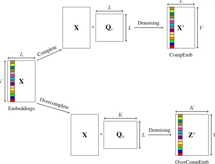
In this section, we present the two contributions of this paper. Figure 1 illustrates our two models to learn denoising for word embeddings. The first model on the top, the complete word denoising embeddings model “CompEmb” (Section 2.1), filters noise from word embeddings X to produce complete word denoising embeddings X∗_{, in which the vector length of X}∗ _{in comparison to X is unchanged after}

denoising (called complete). The second model at the bottom of the figure, the overcomplete word denoising embeddings model “OverCompEmb” (Section 2.2), filters noise from word embeddingsXto yield overcomplete word denoising embeddingsZ∗_{, in which the vector length ofZ}∗_{tends to be greater}

than the vector length ofX(calledovercomplete).

For the notations, letX∈RV×L_{is an input set of word embeddings in whichV is the vocabulary size,}

andLis the vector length ofX. Furthermore,Z∈RV×K_{is the overcomplete word embeddings in which}

Kis the vector length ofZ(K > L); finally,D∈RL×L_{is the pre-trained dictionary (Section 2.4).}

2.1 Complete Word Denoising Embeddings

In this subsection, we aim to reduce noise in the given input word embeddingsXby learning a denoising matrixQc. The complete word denoising embeddingsX∗ are then generated by projectingXintoQc.

More specifically, given an inputX∈RV×L_{, we seek to optimize the following objective function:}

argmin X,Qc,S

V

X

i=1

kxi−f(xi,Qc,S)k+αkSk1 (1)

wheref is a filter;Sis a lateral inhibition matrix; andαis a regularization hyperparameter. Inspired by studies on sparse modeling, the matrixSis chosen to be symmetric and has zero on the diagonal.

X

V

Embeddings

Complete

X

L

Q

L

X

CompEmb

Overcomplete

X

Q

K

Denoising

K

V

Z

OverCompEmb

Figure 1: Illustration of word denoising embeddings methods, with complete word denoising embed-dings at the top, and overcomplete word denoising embedembed-dings at the bottom.

The goal of this matrix is to implement excitatory interaction between neurons, and to increase the convergence speed of the neural network (Szlam et al., 2011). More concretely, the matricesQcandS

are initialized withIandE, which are identity matrices, and the Lipschitz constant:

Qc= _E1D;S=I−_E1DTD

E > the largest eigenvalue ofDT_D

D∈RL×L_{be pre-trained dictionary}

The underlying idea for reducing noise is to make use of a filterfto learn a denoising matrixQc; hence,

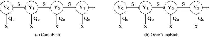
we design the filterfas a non-linear, parameterized, feed-forward architecture with a fixed depth that can be trained to approximatef(X,Qc,S)toXas in Figure 2a. As a result, noise from word embeddings

will be filtered by layers of the filterf. The filterf is encoded as a recursive function by iterating over the number of fixed depthT, as the following recursive Equation 2 shows:

Y=f(X,Qc,S)

Y(0) =G(XQc)

Y(k+ 1) =G(XQc+Y(k)S) 0≤k < T

(2)

Gis a non-linear activation function. The matricesQcandSare learned to produce the lowest possible

Y0

Qc

X

Y1

Qc

X

Y2

Qc

X

Y3

Qc

X (a) CompEmb

Y0

Qo

X

Y1

Qo

X

Y2

Qo

X

Y3

Qo

X (b) OverCompEmb

Figure 2: Architecture of the filters with the fixed depthT = 3.

computational burden (e.g., solving low-rank approximation problem or keeping the number of terms at zero (Gregor and LeCun, 2010)). Moreover, the initialization of the matricesQc,S andE enhances a

highly efficient minimization of the objective function in Equation 1, due to the pre-trained dictionaryD that carries the information of reconstructingX.

The architecture of the filterf is a recursive feed-forward neural network with the fixed depthT, so the number ofT plays a significant role in controlling the approximation ofX∗_{. The effects ofT will}

be discussed later in Section 3.4. WhenQcis trained, the complete word denoising embeddingsX∗are

yielded by projectingXintoQc, as shown by the following Equation 3:

X∗=G(XQc) (3)

2.2 Overcomplete Word Denoising Embeddings

Now we introduce our method to reduce noise and overcomplete vectors in the given input word embed-dings. To obtain overcomplete word embeddings, we first use a sparse coding method to transform the given input word embeddingsXinto overcomplete word embeddingsZ. Secondly, we use overcomplete word embeddingsZas the intermediate word embeddings to optimize the objective function: A set of input word embeddingsX∈RV×L_{is transformed to overcomplete word embeddingsZ∈R}V×K_by

ap-plying sparse coding method in Section 2.4. We then make use of the pre-trained dictionaryD∈RL×K

andZ∈RV×K _{to learn the denoising matrixQoby minimizing the following Equation 4:}

argmin X,Qo,S

V

X

i=1

kzi−f(xi,Qo,S)k+αkSk1 (4)

The initialization of the parameters Qo, S, E and αfollows the same procedure as described in

Sec-tion 2.1, and with the same interpretaSec-tion of the filter architecture in Figure 2b. The overcomplete word denoising embeddingsZ∗ _{are then generated by projectingXinto the denoising matrix Qo and using}

the non-linear activation functionGin the following Equation 5:

Z∗=G(XQo) (5)

2.3 Loss Function

For each pair of term vectorsxi ∈Xandyi ∈Y=f(X,Qc,S), we make use of the cosine similarity

to measure the similarity betweenxiandyias follows:

sim(xi,yi) = _kxxi·yi

ikkyik (6)

Let∆be the difference betweensim(xi,xi) andsim(xi,yi), equivalently∆ = 1−sim(xi,yi). We

2.4 Sparse Coding

Sparse coding is a method to represent vector representations as a sparse linear combination of elemen-tary atoms of a given dictionary. The underlying assumption of sparse coding is that the input vectors can be reconstructed accurately as a linear combination of some basis vectors and a few number of non-zero coefficients (Olshausen and Field, 1996).

The goal is to approximate a dense vector in RL _{by a sparse linear combination of a few columns}

of a matrixD ∈ RL×K _{in which K is a new vector length and the matrixD be called a dictionary.}

Concretely, given V input vectors of L dimensions X = [x1, x2, ..., xV], the dictionary and sparse

vectors can be formulated as the following minimization problem:

min D∈C,Z∈RK×V

V

X

i=1

kxi−Dzik₂2+λkzik₁ (7)

Z= [z1, ..., zV]carries the decomposition coefficients ofX= [x1, x2, ..., xV]; andλrepresents a scalar

to control the sparsity level ofZ. The dictionaryDis typically learned by minimizing Equation 7 over input vectorsX. In the case of overcomplete representationsZ, the vector lengthKis typically implied asK=γL(γ >0).

In the method of overcomplete word denoising embeddings (Section 2.2), our approach makes use of overcomplete word embeddingsZas the intermediate word embeddings reconstructed by applying a sparse coding method to word embeddingsX. The overcomplete word embeddingsZare then utilized to optimize Equation 4. To obtain overcomplete word embeddingsZand dictionaries, we use theSPAMS package2_{to implement sparse coding for word embeddingsXand to train the dictionariesD.}

3 Experiments

3.1 Experimental Settings

As input word embeddings, we rely on two state-of-the-art word embeddings methods: word2vec (Mikolov et al., 2013) and GloVe (Pennington et al., 2014). We use the word2vectool3 and the web corpusENCOW14A(Sch¨afer and Bildhauer, 2012; Sch¨afer, 2015) which contains approx-imately 14.5 billion tokens, in order to train Skip-gram models with 100 and 300 dimensions. For the GloVe method, we use pre-trained vectors of 100 and 300 dimensions4 _{that were trained on 6 billion} words from Wikipedia and English Gigaword. Thetanhfunction is used as the non-linear activation function in both approaches. The fixed depth of filterT is set to 3; further hyperparameters are chosen as discussed in Section 3.2. To train the networks, we use theTheanoframework (Theano Develop-ment Team, 2016) to impleDevelop-ment our models with a mini-batch size of 100. Regularization is applied by dropouts of 0.5 and 0.2 for input and output layers (without tuning), respectively.

3.2 Hyperparameter Tuning

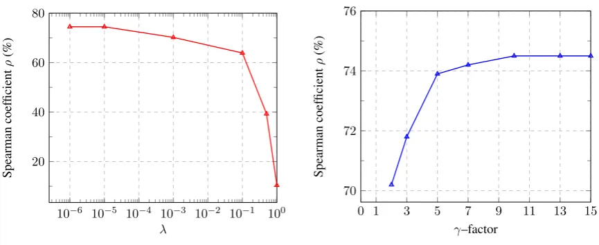
In both methods of denoising word embeddings, the`1regularization penaltyαis set to 0.5 without tun-ing in Equation 1 and 4. The method of learntun-ing overcomplete word denoistun-ing embeddtun-ings relies on the mediate word embeddingsZto minimize the objective function in Equation 4. The sparsity ofZdepends on the`1regularizationλin Equation 7; and the length vectorKofZis implied asK =γL. Therefore, we aim to tuneλandγsuch thatZrepresents the nearest approximation of the original vector represen-tationX. We perform a grid search onλ ∈ {1.0,0.5,0.1,10−3_,10−6_{}andγ ∈ {2,3,5,7,10,13,15},} developing on the word similarity task WordSim353 (to be discussed on Section 3.3). The hyperpa-rameter tunings are illustrated in Figures 3a and 3b for sparsity and overcomplete vector length tuning, respectively. In both approaches, we setλto10−6_{andγto 10 for the sparsity and length of overcomplete} word embeddings.

10−6 ₁₀−5 ₁₀−4 ₁₀−3 ₁₀−2 ₁₀−1 ₁₀0 20

40 60

λ

Spearman

coef

ficient

ρ

(%)

(a) Sparsity of sparse coding.

0 1 3 5 7 9 11 13 15 70

72 74

γ–factor

Spearman

coef

ficient

ρ

(%)

(b) Length of overcomplete vectors.

Figure 3: Illustration of hyperparameter tuning.

3.3 Effects of Word Denoising Embeddings

In this section, we quantify the effects of word denoising embeddings on three kinds of tasks: similarity and relatedness tasks, detecting synonymy, and bracketed noun phrase classification task. In comparison to the performance of word denoising embeddings, we take into account state-of-the-art word embed-dings (Skip-gram and GloVe word embedembed-dings) as baselines. Besides, we also use the public source code5_{to re-implement the two methods suggested by Faruqui et al. (2015) which are vectorsA(sparse} overcomplete vectors) andB(sparse binary overcomplete vectors).

The effects of the word denoising embeddings on the tasks are shown in Table 1. The results show that the vectorsX∗_andZ∗_{outperform the original vectorsX,AandB, except for the NP task, in which the}

vectorsBbased on the 300-dimensional GloVe vectors are best. The effect of the vectorsZ∗ _{is slightly}

less impressive, when compared to the overcomplete vectorsX∗_{. The overcomplete word embeddingsZ}

strongly differ from the word embeddingsX; hence, the denoising is affected. However, the performance of the vectorsZ∗ _{still outperforms the original vectorsX,AandBafter the denoising process.}

3.3.1 Relatedness and Similarity Tasks

For the relatedness task, we use two kinds of datasets: MEN (Bruni et al., 2014) consists of 3000 word pairs comprising 656 nouns, 57 adjectives and 38 verbs. The WordSim-353 relatedness dataset (Finkel-stein et al., 2001) contains 252 word pairs. Concerning the similarity tasks, we evaluate the denoising vectors again on two kinds of datasets:SimLex-999(Hill et al., 2015) contains 999 word pairs including 666 noun, 222 verb and 111 adjective pairs. The WordSim-353 similarity dataset consists of 203 word pairs. In addition, we evaluate our denoising vectors on the WordSim-353 dataset which contains 353 pairs for both similarity and relatedness relations. We calculate cosine similarity between the vectors of two words forming a test pair, and report the Spearman rank-order correlation coefficientρ(Siegel and Castellan, 1988) against the respective gold standards of human ratings.

3.3.2 Synonymy

We evaluate on 80 TOEFL (Test of English as a Foreign Language) synonym questions (Landauer and Dumais, 1997) and 50 ESL (English as a Second Language) questions (Turney, 2001). The first dataset represents a subset of 80 multiple-choice synonym questions from the TOEFL test: a word is paired with four options, one of which is a valid synonym. The second dataset contains 50 multiple-choice synonym questions, and the goal is to choose a valid synonym from four options. For each question, we compute the cosine similarity between the target word and the four candidates. The suggested answer is the candidate with the highest cosine score. We use accuracy to evaluate the performance.

Vectors Simlex-999_Corr. MEN_Corr. WS353_Corr. WS353-SIM_Corr. WS353-REL_Corr. ESL_Acc. TOEFL_{Acc. Acc.}NP

X 33.7 72.9 69.7 74.5 65.5 48.9 62.0 72.8

X∗ _{33.2 72.8 70.6 74.8 66.0 53.0 64.5 78.5}

SG-100 Z∗ _{35.9 74.4 71.2 75.2 68.1 53.0 62.0 79.1}

A 32.5 69.8 65.5 69.5 60.2 55.1 51.8 78.8

B 31.9 70.4 65.8 72.6 62.2 53.0 58.2 74.1

X 36.1 74.7 71.0 75.9 66.1 59.1 72.1 77.9

X∗ _{37.1 75.8 71.8 76.4 66.9 59.1 74.6 79.3}

SG-300 Z∗ _{36.5 75.0 70.6 76.4 64.4 57.1 77.2 78.6}

A 32.9 72.4 67.5 71.9 63.4 53.0 65.8 78.3

B 32.7 71.2 63.3 68.7 56.2 51.0 70.8 78.6

X 29.7 69.3 52.9 60.3 49.5 46.9 82.2 76.4

X∗ _{31.7 70.9 58.0 63.8 57.3 53.0 88.6 77.4}

GloVe-100 Z∗ _{30.0 70.9 56.0 62.8 53.8 57.0 81.0 77.3}

A 30.7 70.7 54.9 62.2 51.2 55.1 78.4 77.1

B 31.0 69.2 57.3 62.3 53.7 46.9 73.4 76.4

X 37.0 74.8 60.5 66.3 57.2 61.2 89.8 74.3

X∗ _{40.2 76.8 64.9 69.8 62.0 61.2 92.4 76.3}

GloVe-300 Z∗ _{39.0 75.2 63.0 67.9 59.7 57.1 86.0 75.7}

A 36.7 74.1 61.5 67.7 57.8 55.1 87.3 79.9

B 33.1 70.2 57.0 62.2 53.0 51.0 91.4 80.0

Table 1: Effects of word denoising embeddings. Vectors Xrepresent the baselines; vectorsA andB were suggested by Faruqui et al. (2015); the vector lengthZ∗_{is equal to 10 times of vector lengthX.}

3.3.3 Phrase parsing as Classification

Lazaridou et al. (2013) introduced a dataset of noun phrases (NP) in which each NP consists of three elements: the first element is either an adjective or a noun, and the other elements are all nouns. For a given NP (such asblood pressure medicine), the task is to predict whether it is a left-bracketed NP, e.g., (blood pressure) medicine, or a right-bracketed NP, e.g.,blood (pressure medicine).

The dataset contains 2227 noun phrases split into 10 folds. For each NP, we use the average of word vectors as features to feed into the classifier by tuning the hyperparameters (w1, w2 andw3) for each element (e1,e2ande3) within the NP:~eNP = 1₃(w1~e1+w2~e2+w3~e3). We then employ the classification of the NPs by using a Support Vector Machine (SVM) with Radial Basis Function kernel. The classifier is tuned on the first fold, and cross-validation accuracy is reported on the nine remaining folds.

3.4 Effects of Filter Depth

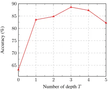
As mentioned above, the architecture of the filterf is a feed-forward network with a fixed depthT. For each stageT, the filterfattempts to reduce the noise within input vectors by approximating these vectors based on vectors of a previous stageT −1. In order to investigate the effects of each stageT, we use pre-trained GloVe vectors with 100 dimensions to evaluate the denoising performance of the vectors on detecting synonymy in the TOEFL dataset across several stages ofT.

0 1 2 3 4 5 65

70 75 80 85

Number of depthT

Accurac

y

(%)

Figure 4: Effects of the filter with depthT on filtering noise.

4 Conclusion

To the best of our knowledge, we are the first to work on filtering noise in word embeddings. In this paper, we have presented two novel models to improve word embeddings by reducing noise in state-of-the-art word embeddings models. The underlying idea in our models was to make use of a deep feed-forward neural network filter to reduce noise. The first model generated complete word denoising embeddings; the second model yielded overcomplete word denoising embeddings. We demonstrated that the word denoising embeddings outperform the originally state-of-the-art word embeddings on several benchmark tasks.

Acknowledgements

The research was supported by the Ministry of Education and Training of the Socialist Republic of Vietnam (Scholarship 977/QD-BGDDT; Kim-Anh Nguyen), the DFG Collaborative Research Centre SFB 732 (Kim-Anh Nguyen, Ngoc Thang Vu), and the DFG Heisenberg Fellowship SCHU-2580/1 (Sabine Schulte im Walde).

References

Heike Adel and Hinrich Sch¨utze. 2014. Using mined coreference chains as a resource for a semantic task. In Proceedings of the 2014 Conference on Empirical Methods in Natural Language Processing (EMNLP), pages 1447–1452, Doha, Qatar.

Elia Bruni, Nam-Khanh Tran, and Marco Baroni. 2014. Multimodal distributional semantics. Journal of Artifical

Intelligence Research (JAIR), 49:1–47.

Manaal Faruqui, Yulia Tsvetkov, Dani Yogatama, Chris Dyer, and Noah A. Smith. 2015. Sparse overcomplete

word vector representations. InProceedings of the 53rd Annual Meeting of the Association for Computational

Linguistics (ACL), pages 1491–1500, Beijing, China.

Lev Finkelstein, Evgeniy Gabrilovich, Yossi Matias, Ehud Rivlin, Zach Solan, Gadi Wolfman, and Eytan Ruppin. 2001. Placing search in context: The concept revisited. InProceedings of the 10th International Conference on the World Wide Web, pages 406–414.

Karol Gregor and Yann LeCun. 2010. Learning fast approximations of sparse coding. InProceedings of the 27th

International Conference on Machine Learning (ICML), Haifa, Israel, pages 399–406. Zellig S. Harris. 1954. Distributional structure. Word, 10(23):146–162.

Felix Hill, Roi Reichart, and Anna Korhonen. 2015. Simlex-999: Evaluating semantic models with (genuine) similarity estimation. Computational Linguistics, 41(4):665–695.

Yoon Kim. 2014. Convolutional neural networks for sentence classification. InProceedings of the 2014

Thomas K. Landauer and Susan T. Dumais. 1997. A solution to Platos problem: The latent semantic analysis theory of acquisition, induction, and representation of knowledge. Psychological Review, 104(2):211–240. Angeliki Lazaridou, Eva Maria Vecchi, and Marco Baroni. 2013. Fish transporters and miracle homes: How

com-positional distributional semantics can help NP parsing. InProceedings of the 2014 Conference on Empirical

Methods in Natural Language Processing (EMNLP), pages 1908–1913, Doha, Qatar.

Tomas Mikolov, Wen-tau Yih, and Geoffrey Zweig. 2013. Linguistic regularities in continuous space word

rep-resentations. In Proceedings of the 2013 Conference of the North American Chapter of the Association for

Computational Linguistics: Human Language Technologies (NAACL), pages 746–751, Atlanta, Georgia. Kim Anh Nguyen, Sabine Schulte im Walde, and Ngoc Thang Vu. 2016. Integrating distributional lexical contrast

into word embeddings for antonym-synonym distinction. In Proceedings of the 54th Annual Meeting of the

Association for Computational Linguistics (ACL), pages 454–459, Berlin, Germany.

Bruno A. Olshausen and David J. Field. 1996. Emergence of simple-cell receptive field properties by learning a sparse code for natural images. Nature, 381(6583):607–609.

Jeffrey Pennington, Richard Socher, and Christopher D. Manning. 2014. Glove: Global vectors for word

rep-resentation. In Proceedings of the 2014 Conference on Empirical Methods in Natural Language Processing

(EMNLP), pages 1532–1543, Doha, Qatar.

Nghia The Pham, Angeliki Lazaridou, and Marco Baroni. 2015. A multitask objective to inject lexical contrast into distributional semantics. InProceedings of the 53rd Annual Meeting of the Association for Computational Linguistics (ACL), pages 21–26, Beijing, China.

Roland Sch¨afer and Felix Bildhauer. 2012. Building large corpora from the web using a new efficient tool chain. In Proceedings of the 8th International Conference on Language Resources and Evaluation, pages 486–493, Istanbul, Turkey.

Roland Sch¨afer. 2015. Processing and querying large web corpora with the COW14 architecture. InProceedings

of the 3rd Workshop on Challenges in the Management of Large Corpora, pages 28–34, Mannheim, Germany.

Sidney Siegel and N. John Castellan. 1988. Nonparametric Statistics for the Behavioral Sciences. McGraw-Hill,

Boston, MA.

Arthur D. Szlam, Karol Gregor, and Yann L. Cun. 2011. Structured sparse coding via lateral inhibition.Advances in Neural Information Processing Systems (NIPS), 24:1116–1124.

Theano Development Team. 2016. Theano: A Python framework for fast computation of mathematical expres-sions. arXiv e-prints, abs/1605.02688.

Peter D. Turney. 2001. Mining the web for synonyms: PMI-IR versus LSA on TOEFL. InProceedings of the

12th European Conference on Machine Learning (ECML), pages 491–502.