Thermal Stratification Stress Estimation using Inverse Method
Kiminobu Hojo 1), Itaru Muroya 1) and Sigeki Suzuki 2)
1) Takasago R&D Center, Mitsubishi Heavy Industries, Ltd. 2-1-1 Shinhama, Arai-cho, Takasago 676-8686, JAPAN
2) Kobe Shipyard and Machinery works, Mitsubishi Heavy Industries, Ltd. 1-1 Wadasaki-cho, 1-chome, Hyogo-ku, Kobe 652-8585, JAPAN
ABSTRACT
In this paper, assuming superimposing the wide-area and the local-area temperature change of a pipe, the thermal stratification stress estimation system was developed from measurement of the outer surface temperature. The wide-area temperature change is assumed to be accompanied by the temperature distribution change. From database based on the steady state heat transfer and thermal stress analysis, the stress change in wide-area is calculated. The local-area stress change is calculated by the inverse method using Green's function of axisymmetric model.
In order to confirm the accuracy of this method, three-dimensional FE analysis was carried out. As a result the stress by the estimation system conservatively agreed with that from FE analysis within 20%.
1. I N T R O D U C T I O N
Thermal fatigue is one of the most important degradation issues for nuclear heavy components. Recently primary coolant leak from the components caused by thermal stratification occurred in several power plants. In 1989, this phenomenon occurred in RHR Suction line of Genkai Unit 1, and in the excess letdown line of Mihama Unit2 [1], [2]. Also in the US leaks occurred from the weld joint between the first elbow downstream of the loop nozzle and the horizontal pipe in a cold leg drain line of Three Mile Island and Oconee[2]. Moreover, in 1999 a reactor coolant leak happened at the connecting pipe and the outer cylinder of the heat exchanger of Tsuruga Unit 2. On this component it was estimated that superimposing long and short cycle temperature changes caused more than ten thermal fatigue cracks [3].
In these situations, in order to maintain integrity of nuclear power plants, it is useful to monitor the temperature change of a power plant and estimate the fatigue damage. Until now several temperature monitoring or fatigue monitoring system have been developed in the US, European countries and Japan[4-7]. Most of these systems utilize the plant data that come from the instruments already installed. They have to take many conservative assumptions to estimate fatigue damage at the focused location where is far from the instrument locations. In some cases more precise estimation will be needed to evaluate the stress change or fatigue damage when the outer surface temperatures of pipes or components are directly measured. But the outer surface temperature change of a component is reduced from the inner surface temperature change, so the stress estimation only using the outer surface temperature might be unconservative way.
In this paper, the simplified method was proposed to evaluate the stress change of elbows due to thermal stratification from the outer temperature measurement and the accuracy of the estimated stress was confirmed by comparing with the results by three-dimensional FE analysis.
2. OUTLINE OF THE EVALUATION METHOD
The outline of the evaluation method is shown in Fig1. The evaluation method is mainly composed of two parts. One is related to estimation of the stress range due to the wide-area temperature change. The other is related to estimation of the
SMiRT 16, Washington DC, August 2001
Paper # 1266stress change due to the local-area temperature fluctuation. The procedure of the stress estimation is as follows. 1) Estimation of the temperature distribution
From the outer surface temperature distribution, the relation between the height from the bottom of a horizontal pipe and temperature on the outer surface is obtained. From these time dependent data, the highest position and the lowest position of the boundary between hot and cold water are determined. Based on both temperature distributions, the maximum Width of the temperature change is obtained. The temperature change on the inner surface is estimated from that on the outer surface by using database of axisymmetric heat transfer analysis.
The temperature history of the local area is chosen from the measurement point where the largest temperature change occurs.
2) The stress range due to the wide-area temperature change (A 0-1)
The stress range caused by the wide-area temperature change is obtained by subtracting the steady state stress at the highest position of the boundary from that at the lowest position of the boundary which are calculated by three dimensional FE analysis
3) The stress change due to the local-area temperature change (A 0"2)
The measurement point with the largest temperature fluctuation is chosen as a representative point to estimate the stress change caused by the local-area temperature change. The temperature and stress change history on the inner surface are estimated by the inverse analysis using Green's function from the history of the measurement temperature on the outer surface.
4) The stress change due to the temperature change that does not propagate to the outer surface (A 0"3)
In case of a thick pipe, the temperature change on the inner surface may not propagate to the outer surface. In spite of no observable temperature change on the outer surface, there might be some stress change on the inner surface. The stress level depends on the pipe thickness, the fluctuation period and heat transfer coefficient on the inner surface. The data base of A 0" 3 was prepared by the parametric analysis.
Finally, the total stress change is estimated by summing these stress changes.
3. D E V E L O P M E N T OF THE STRESS ESTIMATION METHOD
3.1 Database of stress change due to the wide-area temperature change (A 0-1)
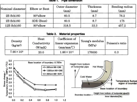
In order to prepare the A 0-1 database typical pipe sizes were chosen from the pipes in which the thermal stratification may occur. The selected pipe sizes are shown in Table 1. Table 2 shows the material properties. The inner and outer surface heat transfer coefficients are 1000 and 1 W/m2K respectively. The steady state stress analyses were carried out with varying the position of the hot-cold water boundary. As an example of the analysis results, the stress range per temperature change on the inner surface is shown in Fig.2. From this figure, it is clear that the larger pipe size gives the larger stress change.
(1) Effect of the pipe size
I Measured temperature on a pipe outer surface I
t
o The highest position of interface • The lowest position of interface
Relation between height from bottom of horizontal pipe and temperature
on outer surface of a pipe
E~E ~o"
.(3 (D E._ ~ O O.
• ~ .N { - "6
~
~:::::::::::::::::::::::::: @ Thermocouples ~ e . ~ l i i i i:il___ -- Measuring section
Iii ~ ~ HOtwater ~ili ii : ~ e c t i o n A
/boundary fluctuation
boundar
Outer surface temperature (°C) Cold water
l
x
I Temperature distribution on inner surface in wide area I ~
I Relation between height from bottom of horizontal pipe and temperature on inner surface of a pipe I
Maximum width of temperature boundary ATmax-in
1 ~ ~ / /
! ~ /
E The highest position I E E of boundary ; / /
=o. r.o I i \ I ../-- -
E -~. luctuation range
O
'P--'~ . . . . .
• - ~ N
~ / I /---~.-N;~N;~tpo~.
"0 / I I ofboundaryl~ Temperature on inner Center position of boundary surface of a pipe (°(3)
t
~ 1 Stress boundary due to wide-area temperature change
J Temperature distribution at I 3D-Solod model highest position and lowest position
i
3D-FE steady state analysis I
i
I Stress range A (71 I
The maximum fluid temperature difference in the design condition (A Tmax-f)
ATmax-f = Thot - Tcold Thot • Temperature of hot water Tcold ° Temperature of cold water
'1
Local temperature fluctuation that does not p r o p a g a t e [ ~to outer surface of a pipe (ATnm)
J
Axial symmetrical FEM (unsteady state analysis)Heat transfer
(inner) k Heat transfer _ _ ^ ^'~, ~ (outer)
Tem0e,atu,e
/ " - " / " " ~ change boundary ATmax-f / Adiabatic condition on outer surfaceATout Fluid temperature change
I ATnm= ATmax-f (with ATout< 1°(3) I
I
I
#
Relations between A Tnm and A (73 Relations between ATmax-f and A (73
I Temperature change in local-area I
History of a measurement point I which has the largest temperature change
I
Section A Q)=_
i
I
Time QThermocouples o
t
H Stress fluctuation due to local-area temperature change ]---
• Estimated by using Green's function
o~- & Outer surface
I t t I t
E ~ ~ I ~
~- Inner ~urface Time Inner surface Time
I Stress change A (72
/
I Total stress range A (7 p
ACT = A(71+ A(72 or A(71+ Ao'2+ A(73
Table 1. Pipe dimension
Nominal diameter
Elbow or Bent
Outer diameter
(mm)
Thickness
(mm)
Bending radius
(mm)
2B Sch160
90°elbow
60.5
8.7
76.2
2B Sch160
3DR (Bent)
60.5
8.7
175
12B Schl60
90°elbow
318.5
33.3
457.2
Table 2. Material properties
Density
(kg/mS)
7.90 × 10⁸
Heat
Conductivity
(W/mK)
20.0
Coefficient of
linear expansion
(mm/mm°C)
1.86 × 10 .5
Young's modulus
(MPa)
176000
Poisson's ratio
0.3
~ 5 . 0 t 4.5 4.0
a.5
,-- 3.0
" ~2.5
O C
~ 2 . 0
I .
~ 1 . 5 ~ 1.0
ID e~
E 0.5 !-
0.0
Base location of boundary" 0.75Din
-O- 2BSch 160-E90
I I I , I I ,
0.0 0.2 0.4 0.6 0.8 1.0
Boundary fluctuation width / [nner diameter 1.2
Boundary location =
Temperature fluctuating region of boundary
. . . n of boundary
Height from bottom of horizontal pipe(H) Inner diameter(Din)
Fig.2 Stress change per temperature change on inner surface
i 12Boioe
W ide temperature fluctuation width
(Small temperature gradient) Narrow temperature fluctuation width (Large t ~ u r e gradient)
( 2 ) Effect of the boundary position
In the case of the 2B pipe, the relation between the base location of the boundary and the temperature fluctuation range on the inner surface is shown in Fig.4. In this case it is assumed that the temperature change of fluid is 100 degree C. Fig.5 shows the relation between the base location of the boundary and the stress fluctuation range on the inner surface. In Fig.5, it is shown that the temperature fluctuation range of the 90 degrees elbow is smaller than that of the bent (3DR) except for the case of the base location of the boundary 1.0. This tendency comes from the shorter temperature fluctuation width of the 90 degrees elbow than that of the bended pipe assuming the same temperature fluctuation width in the vertical direction. When the base level of the boundary is located at the 1.0Din, i.e. the boundary is located at the top of the horizontal pipe, the largest stress change will occur.
( 3 ) Effect of the bending radius
As shown in Fig.2, the effect of the bending radius upon the stress range is small where the boundary fluctuation width is variable and the base location of the boundary is fixed. On the other hand, Fig.5 shows that the bending radius has some effect on the stress level where the boundary location is variable. From this figure, larger bending radius gives larger stress range.
o~ 7o
v
© 60 I=o
t "
=.. 50
t - O
"~ 40 3
0
= 30 ~ 20 ~10 E ~ 0
0.0
-O- 2BSch 160-E90 160-3DR
Fluid temperature fluctuation range" 100°C Boundary fluctuation width :0.1 Din
140
120
o100 b~
~" 80
c- O
".D
~ 60
0
~ 40
o 20 0
-O- 2BSch160-E90 --El- 2BSch160-3DR
Ruid temperature fluctuation range: 100°C
Boundary fluctuation width :0.1 Din
0.5 1.0 1.5 2.0 0.0 0.5 1.0 1.5 2.0
Base location of boundary ( x inner diameter Din) Base location of boundary ( x inner diameter Din)
Fig.4 Relation between base location of boundary and temperature change range on inner surface
Fig.5 Relation
boundary and surface
between base location of
stress change range on inner
3.2 Stress change due to the local-area temperature change (A o'2)
Authors have developed a monitoring system using the inverse method from the outer surface temperature [7]. This system utilizes the Green's function method as an inverse method of heat transfer analysis and as a real time stress calculation caused by thermal stratification change. In this paper, in order to calculate the stress change caused by the local-area temperature change ( A o" 2), the similar function of the monitoring system was installed to the new system.
3.3 Stress change due to the temperature change that does not propagate to the outer surface (A o 3 )
temperature and stress change on the inner surface. By the parametric analyses of fluctuating period, the largest stress changes A 0"3 were chosen. A pipe with larger thickness gives larger stress change comparing with a pipe with small thickness.
120 H e a t t r a n s f e r c o e f f i c i e n t on i n n e r s u r f a c e • 1000 ( W / m 2 K )
100
v ( 1 )
80
e - t -
._o 60
4 - ) ( 0 - t . J 0
= 40
~ 20
L
if)
O 2Bsch 160
- - - _ ~ _ _ _
_ _ _
( 3 ~ r ' , , ,
0
0 20 40 60 80 100 120
Temperature fluctuation range of fluid (°C)
Fig.6 Relations between stress fluctuation range on inner surface and fluid temperature fluctuation range
4. V E R I F I C A T I O N OF T H E P R O P O S E D EVALUATION M E T H O D
In order to confirm the accuracy of the proposed evaluation method, unsteady state heat transfer and thermal stress analysis using three-dimensional model was carried out. The FE model of 12B Schl60 pipe is shown in Fig. 7. The number of nodes and element were 22248 and 18360. The element type was 8-noded brick element. MARC K7.3 was used for FE code. The base level of the boundary was located at 1.0 Din (the inner diameter) and temperature fluctuation width was 0.5 Din with a sine wave with 100sec period.
Fig. 8 shows comparison of temperature change on the inner surface by 3D FE analysis and the estimated temperature change on the inner surface by the inverse method using axisymmetric model. Input data of the inverse method was the outer surface temperature change by 3D FE analysis. Inverse method gives good agreement with 3D FE analysis result.
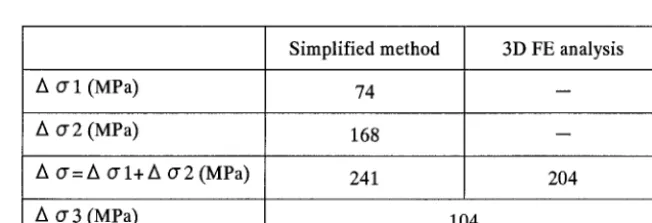
Table3 shows the estimated stresses by the simplified method and those by 3D FE analysis. The total stress by simplified method conservatively agrees with that of FE analysis within 20%.
5. C O N C L U S I O N
Assuming superimposing the wide-area and the local-area temperature change of a pipe, the thermal stratification stress estimation system based on measurement of the outer surface temperature was developed. The wide-area temperature change is assumed to be accompanied by the temperature distribution change. From database based on the steady state heat transfer and thermal stress analysis, the stress change in wide-area is calculated. The local-area stress change is calculated by the inverse method using Green's function of axisymmetric model.
In order to confirm the accuracy of this method, three-dimensional FE analysis was carried out. As a result the stress by the estimation system conservatively agreed with that from FE analysis within 20%.
Fig.7 3D FE analysis model
300
280
260
4" 240
e ~
E ~ 220 I---
200
180
FEM analysis (outer surface) ~ F E M analysis (inner surface) -- -Predicted temperature (inner surface)
i i i
0 100 200 300 400
Time (sec)
Fig,8 Temperature estimation on inner surface by inverse method
Table 3. Comparison of stress by three-dimensional FEM analysis and the simplified method
Acr 1 (MPa) A 0"2 (MPa)
A or= A cr 1+ A 0 2 (MPa) a 0"3 (MPa)
Simplified method 74 168 241
104
3D FE analysis
204
REFERENCES
1. Shirahama, S., "Failure to the Residual Heat Removal System Suction Line Pipe in Genkai Unit1 Caused by thermal Stratification Cycling", Experience with Thermal Fatigue in LWR Piping Caused by Mixing and Stratification, June 8-10, 1998, France, p.73-81.
3. Hoshino, T. et al.,"LEAKAGE FROM CVCS PIPE OF REGENERATIVE HEAT EXCHANGER INDUCED BY HIGH-CYCLE THERMAL FATIGUE AT TSURUGA NUCLEAR POWER STATION UNIT 2", 8 th International Conference on Nuclear Engineering, April 2-6, 2000, Baltimore, MD USA.
4. C.B. Bond and C.C. Barbier, Implementation of a transient and fatigue cycle monitoring program at Virgil C. Plant, ASME PVP 240, 1992.
5. K.A. House and D.A. Gerber, Transient Monitoring Program at Sequoyah Nuclear Plant Units 1 and 2, ASME PVP 240, 1992.
6. K. Sakai, K. Hojo, A. Kato and Umehara, On-line fatigue- monitoring system for nuclear power plant, Nuclear Engineering and Desigin 153, 1994, p19-25.