Copyright 0 1985 by the Genetics Society of America
EVOLUTION AND EXTINCTION OF TRANSPOSABLE
ELEMENTS
I N MENDELIAN POPULATIONS
NORMAN KAPLAN, TOM DARDEN AND CHARLES H. LANGLEY
Biometry and Risk Assessment Program and Laboratory of Genetics, National Institute of Environmental Health Sciences, Research Triangle Park, North Carolina 27709
Manuscript received December 30, 1983 Revised copy accepted October 18, 1984
ABSTRACT
A model of the evolution of a transposable element family in a Mendelian host population is proposed that incorporates heritable phenotypic mutations in the elements. The temporal behavior of the numbers of mutant and wild- type elements is studied, and the expected extinction time of the transposable element family is examined. Our results indicate that, if the mutant can be transposed equally well in the presence of the wild type, then it can be expected to be found in preponderance, whereas elements, such as retroviruses, where the transposing genome and its phenotypic expression are coupled, may be characterized by a low mutant frequency.
ENETIC variation among members of a transposable element family in
G
metazooans is common (see SPRADLING and RUBIN 1981; Jelinek andSCHMIDT 1982 for reviews). In Drosophila, P, FB and l O l F elements are examples in which copies are typically structurally heterogeneous (RUBIN KID-
WELL and BINGHAM 1982; BINGHAM, KIDWELL and RUBIN 1982; ENGELS 1983; TRUETT, JONES and POTTER 1981; LEVIS, COLLINS and RUBIN 1982; PARDUE
and DAWID 1981; DAWID et al. 1981). T h e copia-like elements, in contrast, are considerably more homogeneous but still frequently show size variation due to insertions or deletions (SPRADLING and RUBIN 1981; SCHERER et al. 1982). In vertebrates the AZu and K p n families, which may be transposable elements, are quite variable in size (DEININGER et al. 1981; ADAMS et al. 1980). T h e retro- viruses, which are similar to copia-like elements in that their genome is more conserved in size and structure, also have insertion-deletion variation (CHAT-
TOPADHAY et al. 1982; KHAN, ROWE and MARTIN 1982; RAPASKE et al. 1983).
Some evidence is now available to suggest that the variants in several of these families may be functionally different (SPRADLING and RUBIN 1982; O’HARE
and RUBIN 1983; Weinberg 1980; KHAN, ROWE and MARTIN 1982; REPASKE
et al. 1983). Thus, the genetic variation within families of elements may be an important consideration in understanding the evolution of transposable ele- ments and their effect on the host.
In this paper a model describing the evolution of a family of transposable elements is proposed which allows mutation to functionally distinct mutant elements. This model is a modification of the one proposed by LANGLEY,
460 N. KAPLAN, T . DARDEN AND C. H. LANGLEY
BROOKFIELD and KAPLAN (1983). It is assumed that the host population is a finite, randomly mating Mendelian population of size N . Within the genome of each host there are presumably a large number of locations at which new copies of the element can be inserted, so that when transposition occurs (rep- licatively) it is to a previously unoccupied site. Transposition is considered to be copy number dependent, i.e., in hosts with few copies transposition is more likely than in hosts with many copies. Also, the population dynamics of a newly occupied site are assumed to be independent of the dynamics of all other existing sites. This assumption is reasonable if occupied sites in the population are loosely linked.
T h e new aspect of the model is that there are two possible types of elements at any particular site, the wild type and the mutant. Each generation the wild type can delete or mutate, whereas the mutant can only delete. Two differ- ences between the wild type and the mutant are accounted for in the model. First, the mutant may have a different deletion rate and, second, the mutant may not be able to transpose as efficiently as the wild type.
Unlike other models describing the evolution of transposable elements (LANGLEY, BROOKFIELD and KAPLAN 1983; CHARLESWORTH and CHARLES- WORTH 1983), the proposed model predicts that the element will go extinct. In this paper we study the behavior of the time until extinction and the dynamics of the process until extinction occurs.
THE MODEL
A family of transposable elements will consist of t w o types of elements, the wild type and the mutant. A location in the genome at which either a wild type or mutant is found in at least one of the N genomes in the population is called a site. T h e first assumption of the model is that the frequency process of a site has the same stochastic structure as a three-allele Wright-Fisher process with deletion and mutation, i.e., if in generation t the population frequencies of the wild
type
and the mutant at a particular site arefi(
1 ) andfi(2),
respec- tively, then the joint distribution of J+l(l) andfi+1(2)
conditioned on fi(1) andfd2)
iswhere
and
4 3 = 1
-
( 1-
S l K ( 1 )-
(1-
62K(2).EVOLUTION OF TRANSPOSABLE ELEMENTS 461
T h e second assumption of the model is about the transpositional mechanism for introducing new sites into the population. Since there are a large number of possible locations in the genome at which new copies can be placed, it is assumed that each new copy is inserted at a location that is currently unoc- cupied in the population. Two essential features are incorporated in the sto- chastic structure governing the numbers of new sites introduced by transposi- tion. First, the transposition process is assumed to be copy number dependent,
i.e., when there are few copies (mutant and/or wild type) in the genome, the conditions are more favorable for the creation of new copies than if there are many copies in the genome. Second, a mutant cannot transpose as efficiently as a wild type. In particular, it will be assumed that a wild
type
must be present in the genome for the mutant to transpose.A general way to model this process is the following. Each generation ran- dom numbers of wild type and mutant are created in each of the N host daughters. Let J ( l ) ,
. .
.
, J(N) denote these random quantities, where J(i) =(J( 1 ,
i),
J(2,i))
and J( 1,i)
and J(2,i)
are the numbers of wild type and mutant created in the ith daughter. It is assumed that the J’s are independent, iden- tically distributed random vectors and that their common distribution depends only on the random quantities { p ( i , j ) ,i,
j 2 01, where p ( i , j) is the fraction of the parent population havingi
wild type and j mutant copies. Since the p ( i , j )change from generation to generation, they will be written as pt(i, j ) to denote the generation. Similarly, the J’s are written as Jt(l),
. . .
, J@). T o simplify notation Jt will denote any of the Jt( .).T h e following assumptions will be made about the distribution of Jt. T h e daughters of each generation are formed by randomly choosing either N or
462 N. KAPLAN, T . DARDEN AND C. H. LANGLEY
and
K(g9 b ) = .(g
+
b)w(g/(g
+
b))(b/(Bg+
b)).T h e distribution Jt can be obtained by summing over all possible choices of
g
and b. Indeed,where
( E [ p t ( i l ,
id1
if the population is haploidE [ p , ( l , , l2)f1@1, k 2 ) J if the population is diploid. l l + k l = i l
12+k2=i2
T h e final assumption of the model is that the frequency process of a given site evolves in a random way independent of the dynamics of all other existing sites. Strictly speaking, this assumption requires free recombination between sites. It is conjectured that this assumption is reasonable when there is a mod- erate amount of recombination. Simulation results in LANGLEY, BROOKFIELD and KAPLAN (1 983) and CHARLESWORTH and CHARLESWORTH (1 983) support this conjecture.
T h e description of the model is now complete except for the initial condi- tions. For simplicity, it is assumed that the process is started with one wild type which is randomly located in one of the N genomes.
T h e process that has just been described can be formulated as a countable state Markov chain (see appendix 1 in LANGLEY, BROOKFIELD and KAPLAN 1983). Also, since no immigration is allowed, this process will go extinct with probability one; that is, the transposable element will eventually be lost from the population. Let T denote the time to extinction. A new element will usually
either go extinct in a few generations or will establish itself in the population and then go extinct after a large number of generations. T h e probability that extinction occurs in a few generations can easily be estimated (see APPENDIX 1). T h e behavior of the expectation of 7 , given that the element does establish
itself in the population, is more complex and will be studied in the next section.
THE EXTINCTION TIME
It is shown in APPENDIX 2 that, if the population frequencies of wild type and mutant at individual sites are low, then the numbers of wild type and mutant in a randomly chosen gamete are approximately independent Poisson variables whose means are
1
N
EVOLUTION OF TRANSPOSABLE ELEMENTS 463
and
1
N
h ( 2 ) = - (total number of mutant in the population).
T h e recent data of MONTGOMERY and LANGLEY (1983) suggest that in Dro-
sophila melanogaster this condition holds for the three elements they examined:
copia, 297 and 412. T h e sample distributions of the number of copies of copia
and 412 in the
20
X chromosomes surveyed by MONTGOMERY and LANGLEYare consistent with the Poisson approximation, whereas that for 297 is not. T h e variables h(1) and h(2) change each generation and so they will be written as &(l) and Af(2). Since the process
A, =
(Af(l), h , ( 2 ) ) is more conven- ient for studying the extinction time, its behavior will be considered. If the numbers of wild type and mutant in a randomly chosen daughter are taken to be independent Poisson variables, then the conditional means and variances ofAA,(l) = At+l(l)
-
&(I) and AAt(2) = A,+1(2)-
h42)
can be expressed asE[Aht(1)
I
&(I), 4 2 ) ] = - ( a 1+
p)ht(l)+
H*(ht(l), ht(2)),E[Aht(2)
I
hX1), AX2)] =-&&(2)
+
pAt(1)+
K*(AX1),&(e)),
(1)
( 2 )
(3) 1
uz[A&(l)I&(l), &(2)] x [(I
-
61-
~ ) & ( 1 )+
H*(&(l), &(2))]and
1
u2[A&(2)
I
AX1), M 2 ) ] [(I-
&)&(2)+
&(I)+
K*(ht(l), &(2))], (4)where
Ai( 1) Aj(2)
H*(h,(l), At(2)) =
z
e-(A~1)+AX2))-
-
H ( i , j )i j
i!
j !and
Equations (1)-(4) are consistent with the assumption that mutation deletion and transposition all occur simultaneously. If mutation and deletion occur before transposition, then &(l) and &(2) in equations (1)-(4) need to be re- placed by A,(l)(l
-
p-
61) and h,(2)(1-
&)
+
A,(l)p, respectively. If p,&
are small, then the quantitative, as well as the qualitative, results in both cases are essentially the same.
T h e important observation is that for large N, the conditional variances of
AA,(l) and Aht(2) given in (3) and (4) are small compared to their conditional means given in (1) and (2). Markov processes with negligible conditional vari- ances have been studied by many authors (KURTZ 1971; NORMAN 1975; BAR-
464 N. KAPLAN, T. DARDEN AND C. H. LANGLEY
trajectories of the At process are with high probability very close to the solution of the following system of difference equations:
xk+1
-
xk = -(a1+
p)xk+
H*(Xk, yk)(xo, yo) =
(;
9 0).If the system of difference equations in ( 5 ) has a globally attracting fixed point, (xm, ym), then for all values of N the solution of this system of difference equations will converge to this point. Thus, when N is large, the expected value of 7 1 , the time that it takes the
A,
process to first enter a small neigh- borhood of (xm, p,), can be approximated by 71, the time it takes for the solution of the system of difference equations in ( 5 ) to first enter this neigh- borhood.T h e question remains how to specify the neighborhood of the fixed point. T h e method by which this is done uses a conditional limit theorem of T.
DARDEN and T. G. KURTZ (personal communication). This result states that, for large N and large t, the distribution of
A,,
given that At(l)>
0, is approx- imately bivariate normal with mean vector m = (xm, ym) and covariance matrixQN,
whereQN
= (l/N)Q andQ
is the solution of the matrix equationRQ
+
Q R ~+
A =o
where
R T is the transpose of R and
Fl(X, y) = -(61
+
p ) x+
H * ( x , y)F 2 ( x , y) = -62y
+
px+
K * ( x , y).EVOLUTION OF TRANSPOSABLE ELEMENTS 465 where
r(0.99)
e-xdx = 0.99.
It is of interest to determine the effect of N on ? I . One can show by linearizing the system of equations in (5) in the neighborhood of the fixed point and the origin that is approximately a linear function of logN. Possible exceptions can occur when Xm is near 0. (See discussion of examples later.)
The behavior of the
A,
process after it enters a small neighborhood of the fixed point has also been studied (LUDWIG 1975; BARBOUR 1976; SHUSS 1980). It is possible to show that the expected value of 7 2 , the time until all wild typeare lost from the population (the first time A,(l) = 0), grows exponentially with N . That is, there exists a constant y, not depending on N, such that
The implication of
(7)
is that, when N y is large, it takes an enormous amount of time for all of the wild type to be lost from the population. In general it is difficult to compute y (LUDWIG 1975, 1980). One would expect, however, that xm and are positively correlated so long as Xm+
y m remains constant. Although we cannot prove this in general, the examples of the next section support this conjecture.If xco is close to 0, then y may be so small that eNy may not be large. In this case, 7 3 , the time until the extinction of the mutant, may be relevant. Upon extinction of the wild type, the
A,
process is one-dimensional and can be approximated by a diffusion with drift -&y and variance y / N . For a diffusion with these parameters, the expected absorption time at 0 can be computed explicitly (KARLIN and TAYLOR 1981). If y * is the average number of mutant copies per genome when all wild type delete, thenIt follows from equation (8) that, when &Ny* is large,
1
E(73 I y * )
s,
log(2&2Ny*).Thus, E ( T ~ Iy*) is large if 6 2 is small. It is also clear that E(TS
Iy*)
grows like logN.The analysis just presented can be summarized in the following way. If the process does not go extinct in a few generations, then 7 is the sum of three
components. The first component, 7 1 , is the time needed for the process to enter a small neighborhood of the fixed point, (Xm, ym). The second component,
7 2 , is the additional time necessary for the wild type to go extinct and the final
466 N. KAPLAN, T. DARDEN AND C. H. LANGLEY
N+y is large, then 7 2 is very large, and for most of this time the process is in a
neighborhood of the point (xw, y,). If, on the other hand, N+y is small, then the loss of all wild type from the population can occur in a reasonable number of generations and so the deletion rate of the mutant can have a substantial effect on the expected extinction time.
EXAMPLES
T h e analysis of the behavior of the extinction time requires that the system of difference equations in ( 5 ) have a globally attracting fixed point. Although we have not been able to prove that a fixed point exists for all choices of r , w and
p,
we have been able to prove its existence for all r as defined before,/3 = 1, /3 = 00 and for the following two choices of w:
0 x = o
{
1 x > o(a) ~ ( x ) =
(b) ~ ( x ) = x
If
p
= 1, then the expected proportion of newly transposed copies that are wild type is equal to the proportion of copies in the daughter that are wild type, i.e., the wild type has no selective advantage over the mutant in the transpositional process. On the other hand, ifp
= CQ, then all transposed copiesare wild type. T h e function W I is appropriate when it is envisioned that one wild type generates sufficient gene product for maximal transposition of both the wild type and mutant. T h e function wp corresponds to the case in which each wild
type
produces a small amount of gene product and so the total level of transposition is proportional to the number of wild type in the genome. Even for these special cases we are only able to establish that the fixed point is locally stable. All of the computer results, however, support the conjecture that the fixed point is globally stable. T h e detailed proofs of the existence and uniqueness of the fixed point, and of its local stability for the cases cited, are given in APPENDIX 3.It is of interest to examine for these cases the behavior of the fixed point and the expected extinction time as 61, 6 2 and p vary. T o do this r must be specified. For the rest of this section it will be assumed that ~ ( x ) = l / x if x
>
0 and r(0) = 0.T h e values of x, and y, were found by solving the following equations for appropriate choices of /3, w , 61, 6 2 and p:
and
EVOLUTION OF TRANSPOSABLE ELEMENTS 467
be obtained analytically, and so a computer is needed to find it. For = CO,
some simplification occurs since the expectation in (1 0) disappears. Thus, ym = (p/a2)x,. Equation (9) is still intractable. One should note that (9) is the same for the two cases: w = w l , @ = 1 and w = we and @ = W.
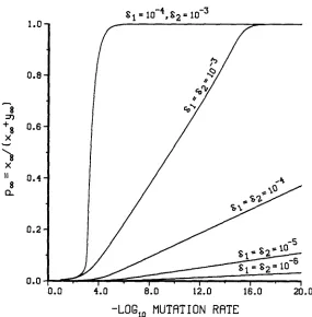
We now examine the behavior of the fixed point. It is convenient for this purpose to define the ratio
pm
= Xm/(Xm+
y,). It is shown in APPENDIX 3 that, if w = w l , and r(x)-
l / x as x + CO, then xm+
ym-
l / ( G ) . Thus, in thiscase the values of Xm and y m can be approximated if
pm
is known. In Figure 1p ,
is plotted as a function of log p, assuming that @ = 1, w = w1 and 6, = 62. T h e cases in which 61 = 62 are in some sense the simplest since it is assumedthat the mutant differs from the wild type only in that it cannot produce the necessary gene products for transposition. For most values of p and 61 = 6 2 ,
p ,
is close to 0, and only when p is unrealistically small canpm
come close to 1. Thus, wild type that mutate in this fashion should be rare during most of the evolution of the element. Selective differences between the mutant and the wild type can modify this conclusion. If 61<
6 2 , then the wild type deletesslower than the mutant, and so
pm
is closer to 1 for larger values of p. This behavior is demonstrated in Figure 1. It is also clear from Figure 1 that, when 6,<
a2,
p,
can be close to 1 for values of p comparable to 61 and 6 2 . O n theother hand, if 62
<
cll, then the wild type deletes faster than the mutant, and so the associatedpm
values should be small, and indeed they are. For example, if 6, = 0.001,a2
= 0.0001 and p = lo-’, then the value ofp ,
is only 0.0035. T h e effect of @ onpm
is also of interest. One would expect on intuitive grounds that increasing @ should favor the wildtype
during transposition and, hence, increasepm.
Unfortunately, we cannot easily computep ,
for any finiteP
other than @ = 1. However, for the limiting case, @ = 03,pm
= & / ( p+
62).It is not difficult to check that in Figure 1 the value of
p ,
for @ = 1 lies below the value ofp m
for @ = 00 for any choice of p , 61 and 62. Furthermore, it isreasonable to expect that the value of
pm
for any @<
1 lies below the value for @ = 1 and that the value ofpm
for any @>
1 lies above the value for @ =1 and below the value for @ = W.
T h e functional form of w can also affect
p,.
T h e function w measures the dependence of overall transposition on wild-type copy number. In particular, the closer w is to 1 the more advantageous it is for the mutant during trans- position. Thus, one would expect smaller values ofp ,
for w1 than for w2.Calculations not given here show this to be the case. Indeed, if
a1
= 62, @ = 1 and w = wp, then p , is close to 1 for values of p comparable to hl.We next consider the behavior of the expected extinction time. Since the qualitative conclusions depend primarily on the location of the fixed point and not on the specific choices of r , w and
p,
we will assume for definiteness that r ( x ) = l/x, x>
0, r(0) = 0 , w = w1 and @ = 1. T h e values of 61, 6 2 and p forthe three examples studied are (lou5, IO-’, lo-’) and (lo-’,
lo-’, respectively. T h e value of xm
+
ym is 32.0 in each case, but the values of X, are 0.1, 2.5 and 4.8, respectively.468 N . KAPLAN, T. DARDEN AND C. H. LANGLEY
1.0
0.8
-
8I )
X
'8 0.6
Y
B
X
" 0.4
8
a
0.2
0.0
FIGURE 1.-The graph of pm = x,/(x,
+
y-) as a function of log j i . In all cases B = 1 andw = w , .
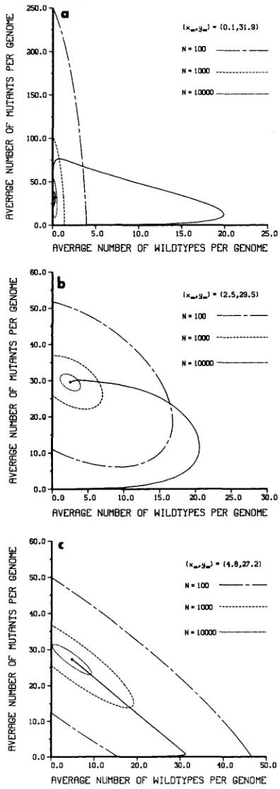
10,000. T h e trajectories of the three examples have essentially the same shape. They appear to have three components. The first part of the trajectory is a rapid buildup of wild type. When the total copy number is sufficiently large, transposition slows down and mutation manifests itself. Finally, as the trajectory nears the fixed point, there may or may not be a spiral effect caused by the competing forces of deletion, mutation and transposition. In Table 1 the values of (measured in generations) are given for the various examples and values of N . Recall that
il
is the time until the trajectory first enters the 99% confi- dence ellipsoid. It is clear from Table 1 that for examples 2 and 3 is approximately a linear function of logN. T h e nonlinear behavior of .?.I for example 1 is due to the unusual shape of the trajectory (Figure 2a).2.7 X and 3.5
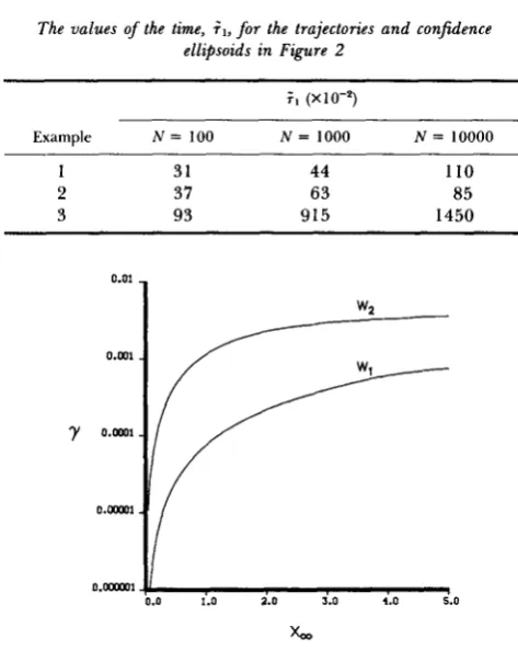
x lo-', respectively. A sketch of how y is computed is given in APPENDIX 4.
T h e value of y increases as xm increases, supporting the conjecture that y and xm are positively correlated so long as xm
+
ym remains constant. More detailed information regarding the relation between and xm is given in Figure 3. Here, y is plotted against xm, assuming that 61 = 62 and xm+
ym = 32. Calcu- lations not given here show that the curve in Figure 3 is essentially the same even if 61 does not equal 62 so long as Xm+
ym = 32. On the other hand, theW E 0 z W W 250.0 m.0- 150.0- LL W Q Q \
\
\
I 1\
L 0 LL W E 3 z m W CII Q LLW >
a W E 0 z W W LL W e 67 c z U c 3 z L 0 LL W E 3 z m W W U LL W > U W x 0 z W W LL W e v) c Z U c 3 z L 0 LL W m
3
z W W (TI LL W > QAVERAGE NUMBER OF WILDTYPES PER GENOME
lx..,gJ
-
l2.5.29.51m*ol
b
N=lm ---
M =
- \
5 0 . 0 - K
_____
~ _________.W . 0 -
'\
'
---._
--..
20.0-
1 0.0 5.0 10.0 15.0 20.0 25.0 ZQ.0
AVERAGE NUMBER OF WILDTYPES PER GENOME
AVERAGE NUMBER OF WILDTYPES PER GENOME
FIGURE 2.-The trajectories of the two difference equations in (5) and the associated 99% confidence ellipsoids. For all examples xo = 0.0 1, @ = 1 and w = W I . For example 1, 61 = 0.0000 1,
6 2 = 0.0001 and p = 0.001; for example 2, 61 = 0.00001, 6 1 = 0.001 and p = 0.001; for example
3, 61 = 0.001, 6 2 = 0.001 and p = 0.00001. The 99% confidence ellipsoids are indicated for N =
100 (- - -), N = 1000 (- - -) and N = 10,000 (. . .).
470 N . KAPLAN, T . DARDEN AND C. H. LANGLEY
TABLE 1
The values of the time, i l , for the trajectories and confidence ellipsoids in Figure 2
;,
(x10-5)Ex amp I e N = 100 N = 1000 N = 10000
1 31 44 110
2 37 63 85
3 93 915 1450
o.mi
y 0.m1
O."l
O. "l
W2
0.0 1.0 2.0 5.0 4.0 5.0
x,
FIGURE 3.-The graph of y as a function xm. In both cases xm
+
ym = 32, 0 = 1 and = 62.The upper curve was computed with w = w , and the lower curve with w = w2.
curve does vary if xm
+
ym is changed. It appears that multiplying xm+
ym by any constant C changes 7 by approximately a factor of C-'. T h e functional form of w can affect these conclusions. In Figure 3 the 7 values are also plotted for w = w2. T h e curve in this case does not rise as quickly, but as before the curve is essentially the same for 61 not equal to 6 2 so long as xm+
ym remains constant. Also, multiplying Xm+
ym by any constant C now changes 7 by approximately a factor ofc - ~ .
T H E SIMULATIONS
T o examine the validity of the results for the expected extinction time, a simulation study was performed. T h e following procedure was used to obtain
A,,, from
A,.
First, the numbers of wild type and mutant in each of the N haploid daughters are independent Poisson variables with meansA,(
1) andEVOLUTION OF TRANSPOSABLE ELEMENTS 471
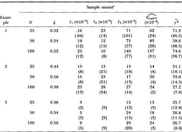
TABLE 2
Simulation results with sampling
Sample means"
A
Exam- EbslP)
-
PIe N
i
i , (x10-2) i z (x10-2) i s (x1o-z) (x10-2) Y*1 25
50
100
2 25
50
100
3 25
50 100 0.52 0.54 0.52 0.44 0.56 0.38 0.56 0.54 0.50 [91 [91 PI 13 18 24 (3) (3) (3) 71.3 (46.5) 58.6 (48.5) 74.6 (36.7) 31.1 (18.1) 33.6 (14.5) 27.2 (7.6) 25.7 (1 2.8) 26.8 (11.5) 26.7 (8.8)
The numbers in parentheses are the sample standard deviations. The numbers in the brackets are the numbers of simulations that exceeded 100,000 generations before the wild type was lost from the population. In those cases was not computed (see text).
For each set of parameter values 50 replicates were performed.
numbers of wild type and mutant in the daughter before deletion and muta- tion. Let
gl
and b! denote the number of wild type and mutant in the ith daughter after the processes of deletion, mutation and transposition have oc- curred. Then,l N I N
N
N
,=I~ i ~ + ~ ( l ) = -
1
gl
and h,+,(2) =-
bl
It was assumed for all simulations that ~ ( x ) = l/x, x
>
0 , r(0) = 0,B
= 1 andw = W I , Furthermore, the simulations were started with ho(1) = 1/N and
ho(2) = 0 and were run for 100,000 generations or until extinction occurred. For each set of parameter values the simulation was repeated 50 times.
472 N. KAPLAN, T. DARDEN AND C. H. LANGLEY
increase as Xm increases. However, since N y is never large, the exponential character of E(72) (equation 6) predicted by the theory is not observed. T h e
estimates of E(73) are consistent with the values obtained from
(7).
T h e simu- lation results also show thaty*,
the average number of mutant copies per daughter when the wildtype
goes extinct, can differ markedly fromym
if xm is small (example 1). On the other hand, if xm is not near 0, theny*
is more centered around ym (examples2
and 3). T h e behavior of y* in example 1 is not surprising in view of the trajectory of the system of difference equations in (5) (Figure 2a). For several of the simulations of example 3, the wild type was still in the population after 100,000 generations (see Table2).
Since the simulation was stopped after 100,000 generations, the values of 7 2 in thesecases are not known, and so there is no way to compute ;z.
It follows from the description of the simulation that each generation the numbers of wild
type
and mutant in the population after mutation and dele- tion, but before transposition, are independent Poisson variables with meansNA,(1)(1
-
61-
p ) and N A , ( l ) p+
NA,(2)(1-
SZ),
respectively. Also the numbers of wild type and mutant created in the population each generation by trans- position are independent Poisson variables with means CJl(g,, 6,) and C&(g,, b,), respectively. Since H and K are nonlinear functions, all of the g,and b, need to be simulated each generation, and so this approach is not feasible if N is large. However, since the (g,, b,) are independently identically distributed, it is reasonable to estimate
C g l H ( g , ,
b,) andC g I K ( g , ,
b,) by 0 ifZ:r”=lg,
= 0 and NE(H(g1,bl))
and N E ( K ( g l , b l ) ) ifCglgI
>
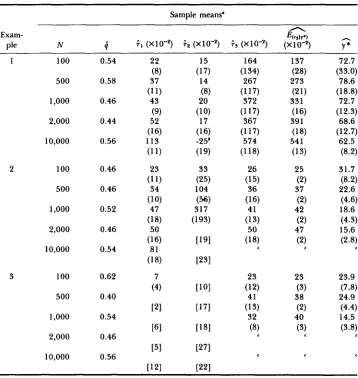
0. In the simulation it was more convenient to replace C$lg, by the number of wild type in the population after deletion and mutation have occurred. If 61 and p are small, this modification has little effect. Although these changes modify the process, the general qualitative features of the original process still remain. In Table 3 the results of the modified simulations are presented for population sizes of 100, 500, 1000, 2000 and 10,000. T h e results for N = 100 are very similar to the results in Table2
for N = 100, suggesting that this pseudosampling scheme does not introduce significant error. T h e values of in Table 3 for examples 1 and 2 agree quite well with the values of 71 in Table 1. T h e values of could not be computed for example 3 since several of the simulations did not enter the 99% confidence ellipsoid before 100,000 generations. This behavior is not surprising in view of the low mutation rate for this example. T h e values of ;Z for example 1 do not show exponential behavior because of the small value of xm. T h e negative entry in the table indicates that the wild type went extinct on average 25 generations before the process entered the 99% confidence ellipsoid. T h e values of ;2 for example 2 do suggest exponen- tial behavior and, in fact, it is possible to estimate y. Let ;2(N) denote the value of ;2, when the population is of size N . Then (7) implies that, for N Z>
EVOLUTION OF TRANSPOSABLE ELEMENTS 473
TABLE 3
Simulation results with pseudosampling
1 100 0.54 22 15 164 137 72.7
(8) (17) (134) (28) (33.0)
500 0.58 37 14 267 273 78.6
(1 1) (8) (1 17) (21) (18.8)
1.000 0.46 43 20 372 33 1 72.7
(9) (10) (1 17) (16) (12.3)
2,000 0.44 52 17 367 39 1 68.6
(16) (16) (1 17) (18) (1 2.7)
10,000 0.56 113 -25b 574 54 1 62.5
(1 1) (19) (118) (13) (8.2)
(1 1) (25) (15) (2) (8.2)
(10) (56) (16) (2) (4.6)
(18) (193) (13) (2) (4.3)
(16) [191 (18) (2) (2.8)
2 100 0.46 23 33 26 25 31.7
500 0.46 34 104 36 37 22.6
1,000 0.52 47 317 41 42 18.6
2,000 0.46 50 50 47 15.6
10,000 0.54 81 c c
(18) ~ 3 1
3 100 0.62 7 23 23 23.9
500 0.40 41 38 24.9
1,000 0.54 32 40 14.5
2,000 0.46
10,000 0.56
(4) P O I (12) (3) (7.8)
121 ~ 7 1 (13) (2) (4.4)
[61 [I81 (8) (3) (3.8)
L
[51 ~ 7 1
[I21 [221
The numbers in the parentheses are the sample standard deviations. The numbers in the brackets are the numbers of simulations that exceeded 100,000 generations before either the process entered the 99% confidence ellipsoid or the wild type was lost from the population. In these cases i t or i n were not computed (see text).
' T h e wild type was lost from the population on average 25 generations before the process
' This value could not be computed since the wild type was still in the population after 100,000
For each set of parameter values 50 replicates were performed.
entered the 99% confidence ellipsoid.
generations for all the simulations.
after 100,000 generations and so ;2 was not computable in these cases. An- other interesting feature of Table 3 is the decreasing behavior of y* as N increases; see examples 2 and 3. This phenomenon is predicted by the theory, and in fact, as N increases y * would be expected to continue to decrease
4 74 N. KAPLAN, T . DARDEN AND C. H. LANGLEY
DISCUSSION
T h e analysis suggests that, if an element does not go extinct in the first few generations, then the average copy number per host genome of the wild type increases quickly in the early stages of the element’s evolution and then de- creases slowly as the average copy number of the mutant starts to grow. T h e average copy numbers in the population of the wild type and mutant then appear to stabilize, but ultimately the wild type disappears from the population leaving only the mutant. At this point transposition stops, and the mutant eventually goes extinct due to the forces of deletion and drift. T h e values around which the average copy number of the wild type and mutant stabilize effectively determine the time to extinction. For any reasonable population size, the extinction time is moderate if the average copy number of the wild
type
stabilizes around a value near 0 and quickly becomes enormous as this value increases.A distinguishing feature of copia-like elements in Drosophila is that most copies are complete. In light of this observation, the behavior of the model suggests that either copia-like elements have recently invaded and are in the early stages of their evolution or copia-like elements are ancient, having long and stable evolutionary histories. T h e latter appears more probable since copia- like elements in D. melanogaster are found in related species and are distributed in a phylogenetic rather than an ecological or geographical pattern (MARTIN,
WEIRNASZ and SCHEDL 1983; BROOKFIELD, MONTGOMERY and LANGLEY 1984). In contrast to copia-like elements, copies of P, FB and l O l F elements in Drosophila are typically variant. In addition the P element is found in natural populations of D. melanogaster but is absent from older laboratory strains and strains of related species (BINGHAM, KIDWELL and RUBIN 1982; BROOKFIELD,
MONTGOMERY and LANGLEY 1984). T h e prediction of the model consistent with these observations is that these elements have recently invaded the pop- ulation and will have a short, less stable evolutionary history (KIDWELL 1979).
T h e mode of transposition of retroviruses and probably copia-like elements provides a plausible explanation of the high frequencies of wild type and their evolutionary stability (WEINBERG 1980; FLAVELL and ISH-HOROWICZ 198 1 ;
SCHERER et al. 1982; SHIBA and SAIGO 1983). If most transposition is via an
RNA intermediate genome copy, then mutation might be expected to be greater than if transposition depended solely on DNA replication since RNA
transcription is generally more error prone. However, the critical relationship between the phenotypic expression of a copy (i.e., the function of the transla- tion products of the RNA transcript) and the actual transposing genome (the same RNA transcript) links defective mutant expression with the mutant ge- nome. Thus, one would expect that in this case selection against defective genomes should be severe, i.e., /3
>>
1 . Indeed, the analysis of the model indicates that, if the mutant is equally well transposed in the presence of the wild type(P
= 1) and is not otherwise selected against (61 =a*),
then theEVOLUTION OF TRANSPOSABLE ELEMENTS 475
mediate form (e.g., P element), since little selection can act on the individual element. Conversely, those elements that transpose via an RNA intermediate or transfect via a viral intermediate will be represented more often by func- tional copies.
LITERATURE CITED
ADAMS, J. W., R. E. KAUFMAN, P. J. KRETSCHMER, M. HARRISON and A. W. NIENHUIS, 1980 A family of long reiterated DNA sequences, one copy of which is next to the human beta globin gene. Nucleic Acids Res. 8: 6113-6128.
BARBOUR, A. D., 1974 On a functional central limit theorem for Markov population processes. Adv. Appl. Prob. 6 21-39.
BARBOUR, A. D., 1976 Quasi-stationary distributions in Markov population processes. Adv. Appl. Prob. 8: 296-314.
BINGHAM, P. M., M. G. KIDWELL and G. M. RUBIN, 1982 The molecular basis of P-M hybrid dysgenesis: the role of the P element, a P-strain-specific transposon family. Cell 2 9 995-1004. BROOKFIELD, J. F. Y., E. MONTGOMERY and C. H. LANGLEY, 1984 Apparent absence of trans-
posable elements related to the P elements of D. melanogaster in other species of Drosophila. Nature 3 1 0 330-332.
CHARLESWORTH, B. and D. CHARLESWORTH, 1983 The population dynamics of transposable ele- ments. Genet. Res. 42: 1-27.
CHATTOPADHAY, S. K., M. V. CLOYD, D. L. LINEMEYER, M. R. LANDER, E. RANDS and D. R. LOWY, 1982 Cellular origin and role of mink cell focus-forming viruses in murine thymic lymphomas. Nature 295: 25-3 1.
Ribosomal insertion-like elements in Drosophila melanogaster are interspersed with mobile sequences. Cell 2 5 399-408.
Base sequence studies of 300 nucleotide renatured repeated human DNA clones. J. Mol. Biol. 151:
17-33.
The P family of transposable elements in Drosophila. Annu. Rev. Genet.
Extrachromosomal circular copies of the eukaryotic DAWID, 1. B., E. 0. LONG, P. P. DINOCERA and M. L. PARDUE, 1981
DENINGER, P. L., D. J. JOLLY, C. M. RUBIN, T. FRIEDMANN and C. W. SCHMIDT, 1981
ENGELS, W. R., 1983
17: 315-344.
FLAVELL, A. J. and D. ISH-HOROWICZ, 1981
HARRIS, T., 1963
JELINEK, W. R. and C. W. SCHMIDT, 1982
KARLIN, S. and H. M. TAYLOR, 1981
transposable element copia in cultural Drosophila cells. Nature (Lond.) 292: 59 1-595. The Theory of Branching Processes. Springer Verlag, Berlin.
Repetitive sequences in eukaryotic DNA and their
A Second Course in Stochastic Processes. Academic Press, expression. Annu. Rev. Biochem. 51: 8 13-844.
New York.
KHAN, A. S., W. P. ROWE and M. A. MARTIN, 1982 Martin cloning of endogenous murine leukemia virus-related sequences from chromosomal DNA of Balb/c and AKR/J mice: iden- tification of an em progenitor of AKR-247 mink cell focus-forming proviral DNA. J. Virol.
44: 625-636.
KIDWELL, M. G., 1979 Hybrid dysgenesis in D. melanogaster: the relationship between the P-M
KURTZ, T. G., 1971 Limit theorems for sequences of jump Markov processes approximating
Transposable elements in Mendelian and I-R interaction systems. Genet. Res. 33: 205-217.
ordinary differential equations. J. Appl. Prob. 8: 344-356.
476
LEVIS, R., COLLINS and G. M. RUBIN, 1982 FB elements are the common basis for the instability
LUDWIG, D., 1975 Persistence of dynamical systems under random perturbations. SIAM Rev. 1%
LUDWIG, D., 1980 Escape from domains of attraction for systems perturbed by noise. pp. 549- 569. In: Nonlinear Phenomena in Physics and Biology, Edited by R. H. ENNS, B. L. JONES and S. S. RANGNEKAR. Plenum Press, New York.
MARTIN, G., D. WEIRNASZ and P. SCHEDL, 1983 Evolution of Drosophila repetitive-dispersed
MONTGOMERY, E. A. and C. H. LANGLEY, 1983 Transposable elements in Mendelian populations.
11. Distribution of copia-like elements in natural populations. Genetics 104: 473-483.
NORMAN, F., 1975 Approximation of stochastic processes by Gaussian diffusions, and applications to Wright-Fisher genetic models. SIAM J. Appl. Math. 29: 225-242.
O’HARE, K. and G. M. RUBIN, 1983 Structures of P transposable elements and their sites of insertion and excision in the Drosophila melanogaster genome. Cell 34: 25-35.
PARDUE, M. L. and I. B. DAWID, 1981 Chromosomal locations of two DNA segments that flank ribosomal insertion-like sequences in Drosophila: flanking sequences are mobile elements. Chro- mosoma 83: 29-43.
Characterization and partial nucleotide sequence of endogenous type C retrovirus segments in human chromosomal DNA. Proc. Natl. Acad. Sci. USA 80: 678-682.
RUBIN, G. M., M. G. KIDWELL and P. M. BINGHAM, 1982 The molecular basis of P-M hybrid dysgenesis: the nature of induced mutations. Cell 29: 987-994.
SCHERER, G., C. TSCHUDI, J. PERERA, H. DELIUS and V. PIRROTTA, 1982 B-104, a new dispersed repeated gene family in Drosophila melanogaster and its analogies with retroviruses. J. Mol. Biol. 157: 435-451.
SCHUSS, Z., 1980 Theory and Applications of Stochastic Differential Equations. John Wiley and Sons,
SHIBA, T. and K. SAIGO, 1983 Retrovirus like particles containing RNA homologous to the transposable element copza in Drosophila melanogaster. Nature (Lond.) 302: 1 19-1 24.
SPRADLING, A. C. and G . M. RUBIN, 1981 Drosophila genome organization: conserved and dy- namic aspects. Annu. Rev. Genet. 15: 219-264.
TRUETT, M. A., R. S. JONES and S. S. POTTER, 1981 Unusual structure of the FB family of transposable elements in Drosophila. Cell 2 4 753-763.
VENTZEL, A. D. and M. I. FRIEDLIN, 1970 On small random perturbations of dynamical systems. Usp. Mat. Nauk 25: 3-55.
WEINBERG, R. A., 1980
N. KAPLAN, T. DARDEN AND C. H. LANGLEY
of the wDZL and wc Drosophila mutations. Cell 30 551-565.
605-640.
DNA. J. Mol. EvoI. 1 9 203-213.
REPASKE, R., R. R. O’NEILL, P. E. STEELE and M. A. MARTIN, 1983
New York.
Origins and roles of endogenous retroviruses. Cell 2 2 643-644.
Communicating editor: W. J. EWENS
APPENDIX 1
If dl and p are small, then deletion and mutation play little or no role in the first few genera- tions, and so only sampling and transposition need to be considered. Let Z. denote the total number of copies in the adult population in generation n. The distribution of Z.+l conditioned on
2. can be represented as the sum of two variables. The first component of the sum Y.+1 represents the number of copies in the n
+
1 generation resulting from sampling. It follows from the Poisson assumptions that Y.+l has a Poisson distribution with mean Zm. The second variable of the sumEVOLUTION OF TRANSPOSABLE ELEMENTS 477
approximately Poisson with mean r( l)Y,,+l. Thus, the conditional generating function of Zm+l can be approximated by
E(szm+l I E.) E E(sYa+le-Yn+I(I-*h'(1) I Z.) e-al-=-('-'M'))
and so Z, is essentially a branching process whose offspring distribution has generating function f ( s ) = e-(l-se++(q
I t follows from standard theory (HARRIS 1963) that the probability of extinction q for the branch- ing process is the smallest solution of the equation
- ( I - q e i w d l ) )
Q
= f h )
= eA straightforward calculation shows that, if r(1) = 1 , then q = 0.497 APPENDIX 2
Suppose in generation t there are IQ) sites in the population and for the ith site (1 5 i 5 I Q ) ) let gdt) and b i t ) denote the frequencies of wild t y p and mutant in generation t. Let G(t
+
1) and B(t+
1) denote the numbers of wiM type and mutant in a randomly chosen gamete. Then G(t+
1) and B(t -t 1) can be represented as
W ) I ( 0
i-1 i- I
G(t
+
1) =1
& ) and B(t + 1) = &(t)where
1 if at site i there is a wild type
0 otherwise,
1 if at site i there is a mutant
0 otherwise.
9i(t) iii
%(t) =
Furthermore,
f'((qi(t), i ( t ) ) * (1, 0 ) I 9 1 ) =i gi(t) f'((Vi(t), 6i(t)) (0, 1) I p t ) bi(t)
and
f'((tli(t), 64t)) = (0, 0) I 9 1 ) = 1
-
gi(t)-
bdt),where 2% represents the history of the process up to time t . If the sites are loosely linked, then the conditional joint generating function of G(t
+
1) and B(t+
l ) , E[sc(t+l)r".'+')l3
can be approximated byI-I
Furthermore, if for all E g,(t)
+
b,(t) is small, then4 1 )
n
(1-
g,(t)(l-
s)-
b,(t)(l-
r ) ) = expl- (1-
s)C
gdt)-
(1-
r )Z
bAt)li- I
= expi- (1
-
s)AXl)-
(1-
r)A42)),since A,(l) =
C.
gLt) and A42) = 2 bdt). If N is large, the approximation is not unreasonable since the frequency process of wild type plus mutant at any site is stochastically bounded by a random deletion process with deletion parameter min(&, 69).478 N. KAPLAN, T. DARDEN AND C. H. LANGLEY APPENDIX 3
In this section we prove the existence and local stability of the fixed point for the system of difference equations in (5). We will always assume that @ = 1. The case @ = 00, which is easier, is
handled in the same way.
Theorem 1 : Let ~ ( x ) be a bounded, decreasing function for x > 0. Furthermore, let r(0) = 0 and r(1) > 61
+
p. Then for w equal to either w1 or w2, there exist unique positive values of xm and ymsuch that
-(&
+
p)x.+
E[
r(X+
Y)w-
-
(x:
Y)
x:
Yl = Oand
- 6 2 ~ -
+
pxuc,+
E[
r(X+
Y)w-
-
(x:Y)x:Yl=o
where X and Yare Poisson variables with means xm and y-, respectively.Proof Case 1: w = w1. The key observation is that, if X and Yare independent Poisson variables with means x and y, respectively, then the distribution of X given X
+
Y is binomial with parametersX + Y and x/(x
+
y). Using this observation we haveAlso,
E[r(X
+
Y)]-
e-"E[r(Y)],X + Y
where xlx=ol = 1 if X = 0 and is zero otherwise.
Let H ( x ) = e-' zP1r(j)(xj-'/j!). T o prove the theorem we need to show there exists unique values of xm and ym such that
-(61
+
p)x,+
X m H ( X ,+
y-) = 0- 6 2 ~ -
+
/U-+
~ , H ( X -+
J-) - Y & - ' ~ H ~ ~ ) = 0.(-43)
and
('44)
It is straightforward to show that H is decreasing, if r is decreasing. Since H ( 0 ) = < I ) > 61
+
p,there exists a unique value of x-
+
y- such that H(x,+
y-) = 61+
p. Let zm = xm+
y-. (A4) can then be written asIt remains to show that for zm fixed, there exists a unique value of ym between 0 and zm satisfying (A5). Let H I denote the lefthand side of (A5) and H2 the right. As a function of y-, H I is linear with H 1 ( 0 ) = pzm and H l ( z m ) = (-62
+
61+
p)zm. Also, H2 is convex, increasing with Hz(0) = 0 and H2(zm) = zmH(z,) = ~ ~+
(p). 6Thus, there must exist a unique value of ~ y-, 0 < ym < z-, such that HIb-) = Hzb-).Case 2: w = w2. Arguing just as in Case 1 , we can show that r(X
+
Y )E r(X
[
+
Y)w2-
-
=-
(x:
Y)x:
J
(x+
y)2 E[
x
+
Y]
+(*Y
+ y)l
EVOLUTION OF TRANSPOSABLE ELEMENTS 479
( A l ) and (A2) can now be written as
-(I%
+
p)P,+
Hs(z,)(p,(l - p-))+
P%Sr,(z,) = 0-
p-)+
P m p+
P c J f * ( z m )-
( P+
61)pm = 0 ,('46)
and
('47)
where
A rearrangement of (A6) and (A7) leads to
and
= Gz(zm).
P
p m = 1
-
H,(z-)
+
6 2-
61We need to show that there is a unique zm such that 0 < Gl(zm) = G&) < 1. Since GI increases,
G2 decreases and 0 < GI(0) < Gz(0) < 1 , the existence and uniqueness of zm is guaranteed regardless of the values of p. 61 and 62. This completes the proof of the theorem.
It follows from the properties of the Poisson distribution that H ( x )
-
r(x)/x as x + W. We thus have the following corollary.Corollary: Suppose r(x)
-
x-= as x ---* OD. Then, for w = w1, xm+
ym-
[I/(&+
p)]ll'(L+O)l.We now turn to local stability.
Theorem 2: The fixed point (x-. y-) is locally stable for both the case 1 and case 2.
Prooj We will only consider case 1 since case 2 is proved in a similar way. The functions F1 and F2 in (6) can be written as
F l ( X , y) = -(61
+
p)x+
xH(x+
y)F&, y) = -6zy
+
px+
yH(x+
y)-
ye-'H(y).Let
M =
E:)
--
To prove local stability it suffices to show that the real parts of the eigenvalues of the matrix M
are negative at (x-, y-). T o do this it suffices to show that at (x-, y-) the trace of M is negative and that the determinant of M is positive.
It follows from (A8) that H(xm
+
y-) = p+
61 and y&-"-H(ym) = p(xm+
y-)+
(61-
6 2 ) ~ ~ . Thus,X-P
Y-
trace M =
- -
+
(xm+
ym)H'(xm+
y-)-
ymedH'(ym).480 N. KAPLAN, T. DARDEN AND C. H. LANGLEY
since [r(l
+
2)/(1+
2)]-
[r(l+
1 ) / ( 1+
I ) ] < 0 for all 1 > 0. Thus, trace M < 0. We next show that the determinant of M is positive. We first note that at (x-, y-), a F l / a x = a F l / 8 y . Thus, the determinant of M is equal to (aFl/ax)(aFz/8y-
a F z / a x ) . Since the a F l / a x < 0, it suffices to show that aFz/8y < aF2/ax. A straightforward calculation shows that(-62
+
y A ’ ( x -+
ym)+
H ( x m+
y-)-
e-’-H(y-)-
yme-”-H’(ym))-
aFz-
3
=ay
a x-(/.I
+
y J f ’ ( x m+
ym)+
y&--H(~m)) = 61-
6s-
y..e-’-(Hbm)+
H’b,))
-
e-+&-)< O
since Hbm)
+
H’b,) > 0. This completes the proof of the result.APPENDIX 4
The proof of the exponential behavior of E(72), which is patterned after the arguments in
VENTZEL and FRIEDLIN (1970), is too complicated to present. One consequence of the proof is the following formula for 7. Let
r(t)
= ( 0 1 ( t ) , &(t)) denote any continuously differentiable curve from (x-, ym) to some point on the positive y axis, and define[Fl and FZ are given in (S)]. Then y equals the infimum of all possible values of
I(r).
T o actually compute y, one uses a result from the calculus of variation which asserts that y = u(0, 0) whereu(x, y ) satisfies the Hamilton-Jacobi equation
all all
f
x(z)’
+
f
y&)’
+
F l ( x , y)ax
+
Fz(x, y ) - = 0 .ay
For additional details one should consult LUDWIG (1975, 1980). Due to the singular behavior of