A Time-Frequency Feature Fusion Algorithm Based on Neural
Network for HRRP
Lele Yuan*
Abstract—In this paper, a feature fusion algorithm is proposed for automatic target recognition based on High Resolution Range Profiles (HRRP). The proposed algorithm employs Convolution Neural Network (CNN) to extract fused feature from the time-frequency features of HRRP automatically. The time-frequency features used include linear transform and bilinear transform. The coding of the CNN’s largest output node is the target category, and the output is compared with a threshold to decide whether the target is classified to a pre-known class or an unknown class. Simulations by four different aircraft models show that the proposed feature fusion algorithm has higher target recognition performance than single features.
1. INTRODUCTION
High Resolution Range Profile (HRRP) is a one-dimensional scattering distribution of a target in range along radar Line-Of-Sight (LOS), which is generated by a high resolution range radar [1]. Compared with other radar imaging techniques, HRRP has many advantages, such as short computing time and small memory space needed, so it has been used for noncooperative target recognition for years [2–4].
In order to explore the information contained in the returned radar signal, either the frequency response or the time signature can be used [5, 6]. Furthermore, recent study shows that Time-Frequency Distribution (TFD) has more power when being applied to HRRP target recognition, which can describe the scattering-point of the target in time-frequency domain more accurately [7, 8]. [7] investigated a time-frequency analysis of HRRP based on Gaussian window and decomposed the range profiles by the natural frame representation which can express the physical characteristics of the signal well. [9] jointed the original HRRP and TFD to classify targets which have high robustness. First, they extracted the training database using the original HRRP roughly and then selected a certain percentage of the highest matching samples to perform decision by extracting time-frequency features. One of the problems to use two-dimension TFD as features is redundancy. To solve the problem, the time-frequency matrix of HRRP was reduced by nonnegative matrix factorization, and the HMM was used as a classifier in [10]. [11] extracted the geometric moment of a two-dimensional image, which is translation, rotation and scale invariance.
According to its form, the TFD includes linear frequency transform and bilinear time-frequency transform. However, both linear and bilinear transforms have shortcomings in Radar Automatic Target Recognition (RATR) [12–14]. The size of the window function used in the linear time-frequency transform determines the time and frequency resolutions of TFD. Longer window results in higher frequency resolution but lower time resolution, while shorter window results in the opposite results. On the other hand, there is no resolution problem in bilinear time-frequency transform, but the cross-terms will interfere the results of bilinear transform. [13] got high resolution and weak cross-terms
Received 30 December 2016, Accepted 8 March 2017, Scheduled 13 March 2017 * Corresponding author: Lele Yuan ([email protected]).
TFD by the complementarity of different features. However, ideal TFD of the signal is required for the fusion process which is difficult to obtain in reality. In this paper, we try to find an approach to fuse different TFDs to get a higher target recognition rate.
We compare the effect of different TFDs on target recognition based on HRRP. Then a feature fusion algorithm based on Convolution Neural Network (CNN) is proposed. The fusion algorithm automatically extracts the TFD fusion feature by a CNN. At the same time, we employ a threshold to determine whether the target is from the known target library or not. If the final result is less than the threshold, we consider it to be an unknown target. In addition, we apply this method to low Signal-to-Noise Ratio (SNR) signal to test the robustness of the algorithm.
2. THE TIME-FREQUENCY TRANSFORM OF HRRP
As for HRRP, the frequency changes with time. Since the Fourier transform cannot accurately describe the signal spectrum changes with time, we should add time factor to the transform, i.e., time-frequency transform [14]. Because the scatter characteristics of the real aircraft target are complex, the shield and motion (such as propellers turbines) of the scatter points will cause some damage to the scattering model and make echoes propagate in the range domain. So the TFD of the aircraft HRRP can reflect the target characteristics more accurately and is more beneficial to RATR [15]. Next, we will introduce linear and bilinear time-frequency transforms briefly.
2.1. Linear Time-Frequency Transform
The most basic form of linear time-frequency transform is Short Time-Frequency Transform (STFT), which is defined as in Equation (1).
ST F T(t, ω) =
x(τ)h(τ −t) e−jωτdτ, (1)
wherex(t) is the signal to be analyzed, andh(t) is the window function which is a symmetric function. On the one hand, h(t) is utilized to intercept a certain time interval of the signal, and the smaller the width of h(t) is, the better the time resolution is. On the other hand, to get high frequency resolution, the window function needs to be as long as possible, which contradicts the time domain resolution.
The commonly used window functions include rectangular window, triangular window, Hanning window, Hamming window, Gauss window (Gabor transform), etc. The linear time-frequency transform also includes wavelet decompose, S-transform and other signal decompose algorithms. In this paper, we use Hanning window and Hamming window.
Hanning window:
h(t) = 0.54 + 0.46 cos2πt
τ , |t| ≤ τ
2. (2)
Hamming window:
h(t) = 1 2
1 + cos2πt τ
, |t| ≤ τ
2. (3)
2.2. Bilinear Time-Frequency Transform
Unlike linear time-frequency transform, the signal appears twice in bilinear time-frequency transform, so called bilinear transform. The most fundamental form is Wigner-Ville transform, which is defined as
W V (t, ω) =
x
t+ τ 2
x∗
t−τ
2
exp (−jωτ)dτ, (4)
To reduce the cross-terms, the Cohen distribution introduced a kernel functiong(θ, τ) to perform as a two-dimensional low-pass filter. The general form is
Cx(t, ω) = 1 2π
x(u+τ /2)x∗(u+τ /2) g (θ, τ) e−j(θt+ωτ−uθ)dudτ dθ, (5)
As shown in the equation, the specific form, type and nature of the transform are determined by the kernel function. When g(θ, τ) = 1, the Cohen distribution is changed into Wigner-Ville distribution. There are many other kernel functions, including Born-Jordan, Choi-Williams, etc. In this paper, we use Wigner-Ville distribution and Born-Jordan function as the TFD to be fused. The Born-Jordan kernel function is shown as follows,
g(θ, τ) = 2sin (θτ /2)
θτ . (6)
The HRRP and TFD from a stealth strategic bomber B2 utilized in the simulation with aspect of 86.4◦ is shown in Fig. 1. It can be clearly seen that the STFTs based on the Hanning window and Hamming window are very similar, but the Hamming window contains more information. The edge of the linear transform shown in Figs. 1(b) and (c) is more blurred than the bilinear transform shown in Figs. 1(d) and (e). The cross-term in Wigner-Ville distribution shown in Fig. 1(d) is even higher than the signal term. The Born-Jordan distribution shown in Fig. 1(d) filters the cross-terms through kernel function but loses much more information than other distributions.
Range bin number
0 100 200
Normalized amplitude 0
0.2 0.4 0.6
(a) Normalized HRRP (b) Hanning window STFT
Normalized time
0 0.2 0.4 0.6 0.8 1
Normalized frequency
0.2 0.4 0.6 0.8 1
(c) Hamming window STFT
Normalized time
0 0.2 0.4 0.6 0.8 1
Normalized frequency
0.2 0.4 0.6 0.8 1
(d) Wigner-Ville Distribution
Normalized time
0 0.2 0.4 0.6 0.8 1
Normalized frequency
0.2 0.4 0.6 0.8 1
(e) Born-Jordan Distribution
Normalized time
0 0.2 0.4 0.6 0.8 1
Normalized frequency
0.2 0.4 0.6 0.8 1
Figure 1. The HRRP and the TFD from B2 with aspect of 86.4◦.
3. THE TIME-FREQUENCY FEATURE FUSION METHOD
3.1. Fusion Method
We introduce the Volterra serial into the fusion process, where the single TFD is used as the first-order term, and the product of the single TFD is used as the second-order term. The calculation method can be expressed as,
dij = n
l=1
ρl(dij)l+ n−1
a=1
n
b=a+1
uab(dij)a(dij)b, (7)
where, dij is a type of TFD;ρ and u are the first-order and second-order coefficients, respectively;nis the number of TFDs to be fused. The reason for adding the second-order product term to the fusion process is that when the TFD is multiplied, the signal part will increase due to higher energy, and the interference term will be suppressed due to lower energy. So the multiplication plays an important role in amplifying the signal and suppress the interference.
3.2. CNN for Feature Fusion
The CNN was originally proposed for handwritten digit recognition by LeCun et al. [16] and has experienced resurgence in deep learning which is utilized in image recognition, speech recognition and other fields [17]. [18] applied the CNN to HRRP from multiple monostatic and bistatic radar systems and significantly improved the reliability of the classification.
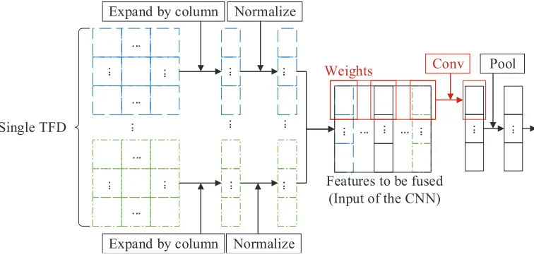
The main idea in CNN is local connection and weight sharing. By using the same weights to scan each part of the image, we can extract the local feature and reduce the number of weights. Every point in the same feature matrix has the same weight coefficient in the feature fusion algorithm. Therefore, the weight coefficients, which are the Volterra coefficients in the previous subsection, can be used as a convolution kernel. The fusion can be achieved by the convolution layer, then the fused features can be classified by the fully-connected layer of the neural network. The architecture of the algorithm is shown in Fig. 2, and the specific implementation is as follows.
Expand by column Normalize
... ...
... ... ...
...
...
...
... ...
...
...
... ...
...
...
...
...
...
...
Single TFD
Features to be fused (Input of the CNN)
...
Conv
Expand by column Normalize
Weights
...
Pool
Figure 2. The architecture of the proposed algorithm. The same line type or color references the same TFD.
First of all, the linear and bilinear time-frequency transforms of HRRP are different in scale, so we should normalize each TFD to the same scale. In this paper, each TFD is normalized to [−0.9,0.9] as follows.
d = 1.8∗(d−dmin) dmax−dmin
+ (−0.9), (8)
where, d and d are the normalized and original TFDs, and dmax and dmin are the maximum and
In order to employ the convolution kernel into feature fusion, we expand each time-frequency matrix by columns and reunite the columns into a new matrix as the network input, i.e.,
D=
⎡ ⎢ ⎢ ⎣
d10 d20 . . . d10∗d20 . . . d1n d2n . . . d1n∗d2n . . .
..
. ... ... . . .
d1N−1 d2N−1 . . . d1N−1∗d2N−1 . . . ⎤ ⎥ ⎥
⎦, (9)
where, D is the input of the network, dmn thenth value of themth TFD expanded by columns, and∗ the product of each two TFDs. Ifn= 0. . . N−1,m= 0. . . M−1, the dimension ofDisN∗(M+C2
M). The convolution layer is utilized to complete the weight fusion process represented by Volterra series. Let the convolution layer consist of K fusion feature maps, and the output of the convolution kernel is represented as
Dck(n) =g(cov (D(n), wk) +bk), (10)
where, n= 0. . . N −1 is the number of a feature row; wk and bk are the kth convolution kernel and bias; cov(·) and g(·) are the convolution and activation function, respectively.
In general, each convolution layer will follow a pooling layer, and the main purpose is to reduce the feature dimension. Because local groups of values are often highly correlated, the pooling operation in local has a certain polymerization which can improve the generalization performance. An average-pooling function of r outputs with stride sis given by Equation (11).
Dpk(l) = (Dck(sl) +Dck(sl+ 1) +. . .+Dck(sl+r−1))/r, (11)
whereDpk(l) is thelth output of the pooling layer followed by thekth kernel andl= 0. . .(N−r)/s. After the convolution and pooling layer, we getK vectors with dimension ofN and then connect all the vectors to a new vectorDfias the input of the full-connected layer. The output of the full-connected layer can be represented as follows,
Dfo =gWTDfi+b, (12)
where,W andbare the weight matrix and bias of the full-connected layer, andg(·) is an active function. The output layer is a fully-connected layer too, and the calculation method is the same as above. The node of the output layer represents the number of classes. Suppose that we have C classes of samples, then the output can be coded asy= [y1, . . . , yC]T. In the desire output, for thecth class, the cth of y is set to 1, and the others are 0.
In this paper, all the active functions are the sigmoid function
g(x) = 1/1 +e−x. (13)
We use the mean square error as the cost function. Letyio and ¯yio represent the actual output of the network and desire output, then the cost functionE can be represented as
E = 1
S S
i=1
C
o=1
(yio−y¯io)2, (14)
where, S is the number of training samples and C the number of output nodes. Then we use Backpropagation algorithm and the stochastic gradient descent method to train the network. In each iteration, the weights, bias, and the convolution kernels are adjusted until the cost function reaches the preset minimum value, or the training epoch reaches the maximum value.
The test sample is prepared as the training sample before input into the trained network. The position corresponding to the maximum output node of the CNN is the class of the test sample. In addition, we introduce a threshold γ ∈[0,1) to classify the target as an unknown target if the highest output does not exceed the chosen threshold, i.e.,
c=
arg max c∈[1,C]
yc, if maxyc ≥γ
unknown, if maxyc < γ , (15)
4. SIMULATION RESULTS
Two-dimensional backscatters distribution data of four different scaled aircraft models are used in the experiment, and the target HRRP is obtained by a stepped frequency radar with a 256-point IDFT in the end. The radar parameters are shown in Table 1. The four aircraft models are B2 (scale 1 : 35), F117 (scale 1 : 13), J6 (scale 1 : 8), and YF22 (scale 1 : 12).
Table 1. Radar parameters.
Parameter Value
Carrier frequency f0 10 GHz
Pulse repetition frequencyfr 100 kHz
Pulse width τ 1µs
Number of pulsesN 256
Stepping frequency increment Δf 1/τ = 1 MHz Resolution ΔR c/(2NΔf) = 0.586 m
The HRRPs are obtained from the aspect range of 0◦ to 180◦ with an equal interval of 0.6◦. From 0◦, every sixth sample, i.e., every 3.6◦, is used for training, and the rest are used for testing. Thus, we have 50 training range profiles and 250 testing range profiles per class. In the training phase, we augment the data by adding white Gaussian noise to obtain the range profiles with 10 dB SNR. The augmented training data set consists of 400 profiles. The testing data set consists of 4000 profiles with SNR varying from 5 to 20 dB with a 5 dB interval and the original profiles.
In this paper, we use four different TFDs of HRRP, including the linear time-frequency transform based on Hamming window and Hanning window, the bilinear time-frequency transform based on Wigner-Ville distribution and Born-Jordan distribution.
First we compare the performance of the proposed feature fusion method and single features. For the single features, we employ a multi-layer neural network as a classifier. Because there is no need to perform fusion, we do not use convolution layer and pooling layer. A fully-connected neural network with the size of 1024-100-4 is to be utilized. The CNN for the feature fusion consists of one convolutional layer with 2 feature maps calculating 1∗10 sample 2D-convolutions followed by a 2-sample average-pooling with stride 2 and a 100-unit fully-connected hidden layer followed by a fully-connected sigmoid output layer. We employ the stochastic gradient descent with momentum, whose learning rate is 0.1, momentum 0.9 and minibatch size 2. The maximum epoch is set at 2000. At first we do not consider the unknown targets, so the threshold γ is set at 0.
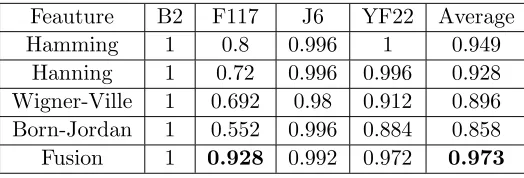
Table 2 shows a comparison of the original profiles classification performance based on different features. The fused feature clearly outperforms the single features, especially for F117. As for F117, all the single features yield a recognition rate below or equal to 0.8, while the recognition rate of the fusion method can be up to 0.9. As for the other three aircraft, both the fusion method and the single features can get high recognition rate, while for the single features, the performance of the linear time-frequency transform is overall higher than the bilinear time-frequency transform.
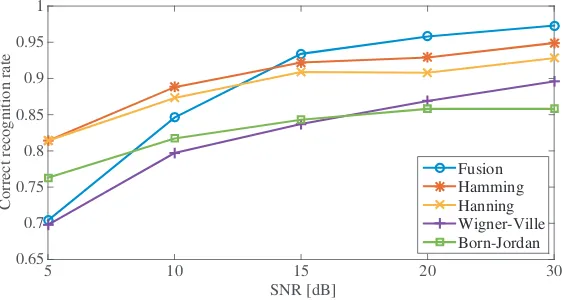
Next we compare the robustness of the proposed feature fusion method and the single features. The recognition rates of different features under different SNRs are compared, as shown in Fig. 3. From
Table 2. The correct recognition rate of different features.
Feauture B2 F117 J6 YF22 Average
Hamming 1 0.8 0.996 1 0.949
Hanning 1 0.72 0.996 0.996 0.928
Wigner-Ville 1 0.692 0.98 0.912 0.896
Born-Jordan 1 0.552 0.996 0.884 0.858
SNR [dB]
5 10 15 20 30
Correct recognition rate
0.65 0.7 0.75 0.8 0.85 0.9 0.95 1
Fusion Hamming Hanning Wigner-Ville Born-Jordan
Figure 3. The recognition rate of different features in different SNR.
Fig. 3, we can see that the fusion method can yield higher performance under high SNR, but under low SNR, the performance drops rapidly. This may be because the target signal is submerged in the noise, and the weighted fusion process also enhances the noise. The confusion matrix for the fusion algorithm under 5 dB SNR is shown in Table 3. Under the condition of low SNR, the F117 is easy confused with other aircraft, and the YF22 is easy confused with F117, so their correct recognition rate is very low, while the other two aircraft still have a high recognition rate. It is because F117 has very high stealth characteristic with little scattering-point, and YF22 has a very similar size and structure to F117.
Table 3. Confusion matrix for the fusion algorithm under SNR = 5 dB.
Declared target
True target
B2 F117 J6 YF22
B2 0.948 0.036 0.004 0.012
F117 0.18 0.5 0.14 0.18
J6 0.04 0.052 0.828 0.08
YF22 0.096 0.24 0.124 0.54
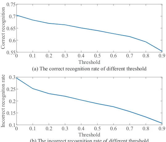
We add a threshold to recognize the aircraft as an unknown class thereby reducing incorrect recognition when the aircraft are confusing with poor condition. We compare the correct rate and incorrect rate under different SNRs and different thresholds. Fig. 4 depicts the correct rate and incorrect rate under 5 dB SNR in different thresholds, and the recognition result of F117 under 5 dB SNR by different thresholds is shown in Table 4. The correct rate and incorrect rate are both decreased with the increase of the threshold, but the incorrect rate decreases rapidly compared to the correct rate of small thresholds. So we can choose a small threshold between [0.1,0.3].
Furthermore, we compare the impacts of different numbers of fused feature maps in the convolution layer. The correct recognition rates of different numbers of feature maps under different SNRs with
Table 4. The recognition result of F117 under SNR = 5 dB by different threshold.
γ B2 F117 J6 YF22 unknown incorrect
0 0.18 0.5 0.14 0.18 0 0.5
0.2 0.108 0.46 0.096 0.16 0.176 0.364
0.4 0.092 0.432 0.084 0.136 0.256 0.312
0.6 0.052 0.412 0.084 0.132 0.32 0.268
Threshold
0 0.1 0.2 0.3 0.4 0.5 0.6 0.7 0.8 0.9
Correct recognition
0.55 0.6 0.65 0.7 0.75
(a) The correct recognition rate of different threshold
Threshold
0 0.1 0.2 0.3 0.4 0.5 0.6 0.7 0.8 0.9
Incorrect recogniton rate 0.1 0.15 0.2 0.25 0.3
(b) The incorrect recognition rate of different threshold
Figure 4. The recognition rate of different features under different SNR.
SNR [dB]
5 10 15 20 free noise
Correct Recognition Rate
0.6 0.7 0.8 0.9 1
2 feature map 4 feature map 6 feature map 8 feature map 10 feature map
Figure 5. The recognition rate of different features under different SNR.
γ = 0.2 are shown in Fig. 5. We can see that under low SNR, the recognition rate can be improved by increasing the number of feature fusion maps until the number is up to 10, because more convolution maps can extract more fusion information from different TFDs.
5. CONCLUSION
In this paper, we compare different TFDs of HRRP and utilize a multi-layer neural network as the classifier to recognize aircraft. By comparing the recognition results, it is found that the linear time-frequency transform is more suitable for target recognition with HRRP. Then we propose the feature fusion algorithm based on TFD which is realized by using a CNN. The recognition result based on the fusion algorithm is much higher than single features under high SNR. To solve the poor recognition result under low SNR, we introduce a threshold to decide whether the target is classified to one of the pre-known targets or unknown targets to reduce the incorrect rate. Furthermore, we find that the recognition rate of low SNR can be improved by increasing the number of feature fusion maps.
REFERENCES
1. Du, L., H. Liu, Z. Bao, and M. Xing, “Radar HRRP target recognition based on higher order spectra,” IEEE Trans. Signal Process., Vol. 53, No. 7, 2359–2368, 2005.
2. Li, H. J. and S. H. Yang, “Using range profiles as feature vectors to identify aerospace objects,” IEEE Trans. Antennas Propag., Vol. 41, No. 3, 261–268, 1993.
3. Wang, J., Y. Li, and K. Chen, “Radar high-resolution range profile recognition via geodesic weighted sparse representation,” IET Radar, Sonar Navig., Vol. 9, No. 1, 75–83, 2015.
4. Zyweck, A. and R. E. Bogner, “Radar target classification of commercial aircraft,” IEEE Trans. Aerosp. Electron. Syst., Vol. 32, No. 2, 598–606, 1996.
5. Kim, K. T., D. K. Seo, and H. T. Kim, “Efficient radar target recognition using the MUSIC algorithm and invariant features,”IEEE Trans. Antennas Propag., Vol. 50, No. 3, 325–337, 2002. 6. Guo, Z. and S. Li, “One-dimensional frequency-domain features for aircraft recognition from radar
range profiles,” IEEE Trans. Aerosp. Electron. Syst., Vol. 46, No. 4, 1880–1892, 2010.
7. Chen, V. C. and D. C. Washington, “Radar range profile analysis with natural frame time-frequency representation,” Proc. SPIE Wavelet Appl. IV, Vol. 3078, 433–448, 1997.
8. Du, L., Y. Ma, B. Wang, and H. Liu, “Noise-robust classification of ground moving targets based on time-frequency feature from micro-doppler signature,”IEEE Sens. J., Vol. 14, No. 8, 2672–2682, 2014.
9. Han, S. K. and H. T. Kim, “Efficient radar target recognition using a combination of range profile and time-frequency analysis,”Progress In Electromagnetics Research, Vol. 108, 131–140, 2010. 10. Zhang, X., Z. Liu, S. Liu, and G. Li, “Time-frequency feature extraction of HRRP using AGR and
NMF for SAR ATR,”Journal of Electrical and Computer Engineering, Vol. 2015, 1–10, 2015. 11. Kim, K., I. Choi, and H. Kim, “Efficient radar target classification using adaptive joint
time-frequency processing,” IEEE Trans. Antennas Propag., Vol. 48, No. 12, 1789–1801, 2000.
12. Thayaparan, T., S. Abrol, E. Riseborough, et al., “Analysis of radar micro-Doppler signatures from experimental helicopter and human data,”Eur. Signal Process. Conf., 289–299, 2006.
13. Lampropoulos, G. A., T. Thayaparan, and N. Xie, “Fusion of time-frequency distributions and applications to radar signals,”J. Electron. Imaging, Vol. 15, No. 2, 1–17, 2006.
14. Sejdic, E., I. Djurovic, and J. Jiang, “Time-frequency feature representation using energy concentration: An overview of recent advances,” Digit. Signal Process. A Rev. J., Vol. 19, No. 1, 153–183, 2009.
15. Guo, Z., D. Li, and B. Zhang, “Survey of radar target recognition using one-dimensional high range resolution profiles,” Systems Engineering and Electronics, Vol. 35, No. 1, 53–60, 2013.
16. LeCun, Y., L. Bottou, Y. Bengio, and P. Haffner, “Gradient based learning applied to document recognition,”Proc. IEEE, Vol. 86, No. 11, 2278–2324, 1998.
17. LeCun, Y., Y. Bengio, and G. Hinton, “Deep learning,”Nat. Methods, Vol. 521, 436–447, 2015. 18. Lunden, J. and V. Koivunen, “Deep learning for HRRP-based target recognition in multistatic