Two-Step Sequential Procedure for the Point Estimation of the Exponential Scale Parameter

ISSN 2286-4822 www.euacademic.org

Impact Factor: 3.1 (UIF) DRJI Value: 5.9 (B+)

Two-Step Sequential Procedure for the Point

Estimation of the Exponential Scale Parameter

EDNA P. ARANGCON – CENITA, M.S.

Southern Philippines Agribusiness, Marine and Aquatic School of Technology Malita, Davao del Sur The Philippines

DAISY LOU LIM – POLESTICO, PHD

Mathematics Department College of Science and Mathematics MSU-Iligan Institute of Technology, Iligan City The Philippines

Abstract:

To estimate the mean



and variance



2_{of an exponential} distribution, Moors and Strijbosch [10] proposed a stopping rule

C

for which the observed sample variance is the extension criterion whether to double the initial sample size

n

_{at the second stage. A modified} two-step sequential procedure for the point estimation of the exponential scale parameter with the inclusion of the cost function to the observed sample variance is proposed. As a measure of accuracy of the procedure, the bias and mean-squared error of the estimates are computed. Also shown is the loss of accuracy due to fixed sample size and estimate of the optimum sample size at stopping.

We derived the estimates and the properties of their mean and the variance. Biases remain in estimating the standard estimators. However, a two-stage sequential sampling plan is recommended to improve accuracy of the estimates of sample of fixed size.

Simulations using the developed Scilab programs are included to illustrate the performance of the procedures in the study.

Key words: Two-Step Sequential Procedure, Point Estimation, Exponential Scale Parameter

1 Introduction

Deciding on the optimal sample size in advance may result to two possibilities; underestimation of the population parameter being estimated or overestimation of the estimates. When

n

is too small, the precision of the estimate can be low, depending on the variance. When

n

is too large, we use unnecessary large number of sample, and face the problem of costly collection of data. Sequential sampling has been developed to address this major problem in sampling. Moors and Strijbosch (2002) studied the two-step procedure in estimating point estimates for gamma distribution. Variance and mean squared error of yas accuracy measures has been explored. In principle, the basic idea to propose such two-stage sequential sampling by Moors and Srijbosch was deeply motivated by the works of Stein (1945), Anscombe (1952) and Chow and Robbins (1965). One may look at Mukhopadhyay et. al. (1994) for a review of sequential estimation theory and method.

In Section 2, we revisit Moors and Strijbosch derivations of all expectations and variances. We propose in Section 3 the stopping variable with the inclusion of cost per unit observation and give formulas for its expected value and variance. In Section 4, we present the expected value, bias, variance and mean squared error of yat stopping. In Section 5, we estimate the variance, bias of the variance, MSE and expectation of

2

s

In Section 6, we present a numerical analysis of Moors and Strijbosch stopping variable and the proposed stopping rule. It is concluded that the modified two-step procedure is a generalization of Moors and Strijbosch procedure for the case of the exponential distribution. It is deduced that when the bound of cost function

c



0.75

, the procedure is effective and

recommended.

2 Preliminary result

Let

X X

₁

,

₂

,...,

X

_n be independent and identically distributed random variables according to an exponential distribution having the probability density function

 

1exp I_ 0_

 

x,

x x

f  x

     





(2.1)

where the scale parameter







0,





is unknown.

Suppose we take a random sample size

n



2

independent

observations x and z from a negative exponential distribution with 2

1

 





. The joint density f_{x z,} ( , )x z is given by

 

 

.

0

,

0

,

,

,

z x

z x z

x

e

z

x

e

z

x

f

 

 









With the transformation for the mean u(xz) / 2 , y x z becomes the deviation between observations.

The Jacobian matrix J of this transformation is

1

u u

x z

J

y y

x z

J

 







_{ }



 



 







_{ }













2

, , , 2

u u y

q u y e y  u

and the conditional densities are derived and given as follows

 





2 1

2

4

,

1

|

,

2

4

u

q u

ue

u

o

q

y u

y

u

u











(2.2)

Now, from the mean

2

x z

u  , we have 2 2

2

y

s



and





2 2

2 2

2

2

2 2

|

2

0

,

2

2

2

s

s

P s

s

u

P

y

o

s

u

u

u











_

 



_











(2.3) Consequently, it follows to derive the conditional density,

marginal density, and conditional expectation.

Differentiating (2.3) with respect to the sample variance 2

s gives us the conditional density given as



2



2 2

2 ₂

1

| , 0 2

8

g s u s u

u s

  

The marginal density of 2

s can be obtained as

 

_{2 2}2 ₂

2

1

, 0

2

s

g s e s

s



 

and the conditional distribution of



and 2 s



₂



₂ 2 _{2 2 2}

|

2

s u

, 0

2

g u s



e





s



u

Consequently, conditional expectation of 2

s given

u

is derived.





2

2 1 2

|

2

3. The Two - Step Sequential Procedure

Given a random sample

X X

₁

,

₂

,...,

X

_n from an exponential population defined in (2.1), we will consider the stopping variable





* 2

1

C



s



cn



w

or





* 2

1

,

1

0

C



s

 

w cn

w cn





where

w

is a predetermined set bound variance on

s

2



cn

₁and 1

n

is the initial sample size. The preselected bound variance 1

w



cn

is chosen in such a way as to achieve some type of balance between sample variability and sampling cost. Motivated by (3.1), the following is the proposed two-step procedure.

First step. Take a random sample of fixed size

n

from an

exponential population defined in (2.1). We compute the sample variance ₁





1



1



1 2

1

1

1

n

n n

i

s

n



x

x











. If it is observed from initial observation that

  

* 2



1

'

C  s  w cn (3.2)

with the inclusion of the cost per unit sample

cn

₁; we terminate sampling; otherwise we proceed to the second step.

Second Step. If the extension criterion holds, we proceed

by recording additional observation, that is, take 1

,

2

,...,

2

n n n

X

_

X

_

X

sample units until

2

n

sample is observed. Thus the final sample size

n

, sample mean

y

and sample variance 2

s is defined





 

'

2 *

1 1 1 2

2 *

3 3 3

,

,

, ,

,

,

n y s

if

C

n y s

n y s

if

C





 

_





Consequently, it follows that





















3 1 2

1 2 3

3 1 2

2

2 2 2

3 3 1 1 2 2 1 2 1 2 3

/

1

1

1

/

n

n

n

y

n y

n y

n

n

s

n

s

n

s

n n

y

y

n

 



















(3.4)

Now, the probability that *

C occurs is

 

* 2w cn1

P C



e

  . The conditional expectation of the mean given the extension criterion as computed as follows



  



  





1

* * 2 2

1 1

|

|

2 2

2

w cn

E u C

P C

E u s g

s

ds

w

cn

p













and



  











1



2 * * 2 2 2

1

1 1

| |

3 2

2

w cn

E u C P C E u s g ds

w cn w cn p



 

   





(3.5)

Noting the consequences of (2.5) and (3.4)









2

*

1 |

4 1 |

2

Var u s Var u C





This result would indicate that variance of the sample mean

u

and variance 2

s is independent of 2

s and the set bound 1

w cn



.

4. Estimation of the Mean

Proposition 4.1: For 2w cn1

p



e

  , with

w



cn

₁

i.

 

4 2



1



4

p w cn

E y   

ii.

 

2



1



4

p w cn B y  

iii.

 

1

3



1

 

1



2

2

8

w cn

w cn p

Var y

 

p









iv.

 

1



3



₁



2 / 8



2

MSE y  p w cn 

Proof: (i) Getting the expected value of (3.3), we have

  

'



 

'





 

3

|

|

E y



E y C P C



E y

C P C

and

  

'



 

'





 

1 1 1

0



E y



E y C P C

|



E y C P C

|

so that

    



 





 

  



 





 





 

  



 





 

   





 

1 1 1 2

1 1 1 2

2 1

1

1 2 1

1

|

|

2

1

=

|

|

|

2

|

|

=

2

1

|

2

E y

E y

E y C P C

E y

y

C P C

E y

E y C P C

E y C P C

E y

C P C

E y

C P C

E y C P C

E y

E y

E y

E y

y C P C

















_



_











From (3.5), the expectation of the estimator

y

is defined,

 



1



1

4 2

, w-cn 0.

4

p w cn

E y    

5 Estimation of the Variance The expectation of 2

1

s can be found similarly. Taking the conditional expectation of (3.3) and applying results of (3.5). However, since only high values of 2

1

s lead to extension of the original sample, it may be expected that 2

s is negatively biased as shown in the next proposition.

Proposition 5.1 For

w



cn

₁, and

n

s

v

2



, we have

i.) 2

3 (

1

)

4

1

(

)

1

6

p w cn

p w cn

E s

  



_











_





;

ii.)

 

2





1 1

3 4 2( )

6

p

B s   _ w cn  w cn _ ; iii.)

 

1 9



₁



10 2



₁



6

2 24

p

E v   _ wcn  wcn  _; and iv.)

 

5 2



₁



12

p

B v   wcn

Proof: (i) To show

 

2

E s , where s2 is the variance of the final sample, perform the expectation of (3.3) and gives

  

2 2





2



1 | ' ( ') 3 | ( )

E s E s C P C E s C P C , 2

1

s is defined as the variance of the initial sample. With the relation

  

2 2





2



1 1 1

0 E s E s |C P C' ( ')E s |C P C( ),

so that



2



  

2 2



1 | ' ( ') 1 | ( )

E s C P C  E s E s C P C . By substitution, we come up with

    



















2 2 2 2

1 1 3

2 2 2

3 1

2 2 2

| ( ) | ( )

= | ( ) | ( )

= | ( )

E s E s E s C P C E s C P C E s C P C E s C P C E s s C P C





  

 

From (3.3), we define





2





2





2





2

3

1

3 1

1

1 2

1

2 1 2 1 2

/

3

n



s



n



s



n



s



n n

y



y

n

. So that,

 

































. 6 2 4 3 1 ) ( | ) ( | 1 1 1 1 2 1 2 2 1 2 2 2 2 1 2 2 1 2 1 2 2 2 2 2 2         _{  }                cn w cn w p C P C s y y s E C P C s y y n n s n s n E s E





The simulated and theoretical values of the estimator y for



yield closer estimates to the parameter being estimated. Overall agreement between the simulated and the true value is observed for the estimator 2

s for



2in Table 4.1.

Table 4.1 Numerical Analysis of the Proposed Sequential Procedure:

Simulation and Theoretical Results when n=500, 2

1

 





simulated TRUE simulated TRUE simulated TRUE simulated TRUE

c = 1 c = 0.1 c= 0.01 c = 0.0001

0.9918 0.9909 0.99437 0.9946 0.99478 0.99334 0.9998 0.9965

 

y

B 0.0082 0.0091 0.0056 0.0054 0.0052 0.0067 0.0002 0.00349

E(s2_{) 0.9703 0.9534 0.9822 0.9745 0.9799 0.9904 0.9994 0.991}

 

2

s

B

0.02973 0.0466 0.0178 0.0254 0.0020 0.0096 0.00500 0.0093

6 Simulation Results

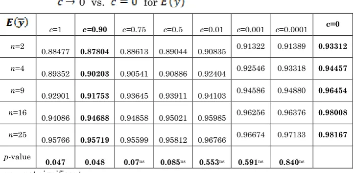
The summary of simulation results are displayed in Table 6 of the two-step sequential sampling design for the parameter values . As the cost is allowed to approach zero, the simulation values are derived from the stopping rule of this study while the simulation results for the column when , are simulation values obtained from the stopping rule of Moors and Strijbosch. The developed Scilab program runs the values when

However, the estimates are closer to the parameter being estimated for larger sample sizes. Furthermore, as the sample size increases, the rate of convergence is faster to the parameter being estimated. Results from t-test at α=0.05 revealed that when

c



0

.

75

, either of the Moors and Strijbosch

procedure or the proposed two – step sequential procedure is applicable . The cost in this case is not negligible but the performance of the procedure is not statistically significant. However, at

c



0

.

75

we cannot neglect anymore the cost of

each observation. The proposed two-step sequential procedure should be used.

Table 6 Numerical Analysis of the Proposed Sequential Procedure as

0 vs. for

c=1 c=0.90 c=0.75 c=0.5 c=0.01 c=0.001 c=0.0001 c=0 n=2

0.88477 0.87804 0.88613 0.89044 0.90835 0.91322 0.91389 0.93312 n=4

0.89352 0.90203 0.90541 0.90886 0.92404 0.92546 0.93318 0.94457 n=9

0.92901 0.91753 0.93645 0.93911 0.94103 0.94586 0.94880 0.96454 n=16

0.94086 0.94688 0.94858 0.95021 0.95985 0.96256 0.96376 0.98008 n=25

0.95766 0.95719 0.95599 0.95812 0.96766 0.96674 0.97133 0.98167 p-value

0.047 0.048 0.07ns _0.085ns _0.553ns _0.591ns _0.840ns

ns – not significant

REFERENCES

[1] Lim, D.L. Isogai E .and Uno C. On the Sequential

Estimation of Functions of Exponential Scale Size Parameters,

(2006).

[2] Moors, J.J.A and Strijbosch, L.W.G. Two - Step Sequential

Sampling for Gamma Distributions, Discussion Paper (2002)

[3] Mukhopadhyay, N. and Zacks, S. Distributions of Sequential and Two-Stage Stopping Times for Fixed-Width Confidence Intervals in Bernoulli Trials: Application in

Reliability, Sequential Analysis, 26:4(2007), 425- 441.