Volume 2010, Article ID 914921,15pages doi:10.1155/2010/914921
Research Article
Fuzzy Morphological Polynomial Image Representation
Chin-Pan Huang
1and Luis F. Chaparro (EURASIP Member)
21Department of Computer and Communication Engineering, Ming Chuan University, Taoyuan 333, Taiwan 2Department of Electrical and Computer Engineering, University of Pittsburgh, Pittsburgh, PA 15261, USA
Correspondence should be addressed to Chin-Pan Huang,[email protected]
Received 8 January 2010; Accepted 7 May 2010
Academic Editor: Srdjan Stankovic
Copyright © 2010 C.-P. Huang and L. F. Chaparro. This is an open access article distributed under the Creative Commons Attribution License, which permits unrestricted use, distribution, and reproduction in any medium, provided the original work is properly cited.
A novel signal representation using fuzzy mathematical morphology is developed. We take advantage of the optimum fuzzy fitting and the efficient implementation of morphological operators to extract geometric information from signals. The new representation provides results analogous to those given by the polynomial transform. Geometrical decomposition of a signal is achieved by windowing and applying sequentially fuzzy morphological opening with structuring functions. The resulting representation is made to resemble an orthogonal expansion by constraining the results of opening to equate adapted structuring functions. Properties of the geometric decomposition are considered and used to calculate the adaptation parameters. Our procedure provides an efficient and flexible representation which can be efficiently implemented in parallel. The application of the representation is illustrated in data compression and fractal dimension estimation temporal signals and images.
1. Introduction
Signal representation is an area of great interest in the signal and image processing. Many representation techniques currently available are well developed and offer satisfac-tory performance in many applications [1–6]. However, in general, drawbacks of these techniques include intensive computation, sequential implementation, and disregard of geometrical information present in signals. In this paper, we propose fuzzy mathematical morphology [7] to represent one- and two-dimensional signals. Fuzzy morphological operators, similar to morphological operator, are nonlinear but well suited for efficient implementation in parallel. Furthermore, they allow to extract geometrical information in signals by appropriate transformations.
Among recently introduced representation techniques, Martens [5,6] proposes a linear combination of polynomial to represent signals. Although the method achieves high performance in data compression, it has high computational complexity and a sequential implementation. Pitas and Venetsanopaulos [8–10] propose a morphological signal decomposition method to decompose a signal into a set of morphologically simple function. Song and Delp [11] use multiple structuring functions instead of a single function
to enhance the performance of morphological filters. In developing the Fuzzy Morphological Polynomial (FMP) representation [12], we take the advantage of polynomial transform idea [5, 6], the morphological decomposition recursive procedures [8–10] and using multiple structuring functions [11] overcoming some of the problems mentioned before.
Binary morphology, as developed in [13], is based on the concept of fitting a structuring element to the signal. Its extension to multilevel morphology was achieved by treating the space underneath the signal (“umbra”) as a binary signal. Recently, Shinha and Dougherty [7] propose an alternate mathematical morphology based on fuzzy set theory. The morphological operations are modeled on a “fuzzy” notion of fitting, the umbra concept is not required and as such binary morphology becomes a special case. The fuzzy fitting yields one or zero for crisp fitting, and between zero and unity for a partial fit. The closer to unity, the higher the degree of fit.
FMP representation are investigated to develop algorithms to compute the adaptive parameters. InSection 4, we extend our algorithm to two-dimensions. We use the tensor product of the two one-dimensional functions as fuzzy structur-ing functions. The order of the two-dimensional fuzzy structuring functions is explored and a rational solution is recommended. InSection 5, we present our experiment results of applying our algorithm to data compression and fractal dimension estimation for one- and two-dimensional signals, demonstrating the advantages of our algorithm. The conclusion is inSection 6. Some of the results in this paper were presented before in [12].
2. Fuzzy Mathematical Morphology
Recently, Shinha and Dougherty [7] proposed to consider fuzzy set theory [14] instead of the classical set theory to develop mathematical morphology. They have in fact, obtained a new approach that considers simultaneously binary and multilevel morphology. The concept of “umbra” is no longer needed to develop the multilevel case. Morpho-logical operations are then developed on the “fuzzy” fitting so that for crisp sets the fitting still remains characterized as either 0 or 1, but for fuzzy or noncrisp sets it is possible to have a fitting characterized by a value between 0 and 1. The closer to unity, the better the fitting of the structuring element. As in the classical morphology, fuzzy morphology [7] also consists in transforming a fuzzy set into another. Such a transformation is performed by means of a fuzzy structuring set containing the desired geometric structure.
If we letXbe the universe of discourse andxbe its generic element, the difference between crisp and fuzzy sets is the characteristic function of a crisp setCwhich is defined asμC: X → {0, 1}while the membership functionμF :X →[0, 1]
of a fuzzy setFis defined so thatμF(x) denotes the degree to
whichxbelongsto the setF. Among the different operations on fuzzy sets [15], the following are important operations to be used later.
(a)Complementoperation:
μFc(x)=1−μF(x). (1)
(b)Translationof a fuzzy setFby a vectorv∈X:
μT(F;v)(x)=μF(x−v). (2)
(c)Reflectionof a setF:
μ−F(x)=μF(−x). (3)
(d)Bold unionof two setsFandG:
μFΔG(x)=min
1,μF(x) +μG(x)
. (4)
(e)Bold intersectionF∇G:
μF∇G(x)=max
0,μF(x) +μG(x)−1
. (5)
The degree of fitting of a setAinto a setBis measured by an inclusion grade operator
I(A,B)=inf
x∈XμA
cΔB(x)
=1 + min0, infx∈X
μB(x)−μA(x)
, (6)
where Δ is the bold union operator. According to the above index, the degree of subsethood of two crisp sets A,Bis either 0 or 1, while for fuzzy sets
CandDI(C,D)∈[0, 1].Moreover, ifC ⊆ Dthen I(C,D) = 1 and in general 0 ≤ I(C,D) ≤ 1. Using such an index [7] has shown that the erosion operation can be defined, and from it the dilation, opening, and closing operators are obtained. In fact, if f(n) is a multilevel and k(n) is a structuring
element with supports F and K and membership
functionμf(n) andμk(n), then we have
Erosion:
μfΘk(n)=I
T(k;n),f
=min
i∈K
min 1, 1−μk(i) +μf(n+i)
, (7)
Dilation:
μf⊕k(n)=μ(fcΘ−k)c(n)
=max
i∈K
max 0,μk(i) +μf(n−i)−1
, (8)
Opening:
μf◦k(n)=μ(fΘk)⊕k(n), (9)
Closing:
μf•k(n)=μ(f⊕k)Θk(n), (10)
2.1. Fuzzification. To apply the above fuzzy morphological operators, the multilevel signal must be converted to its membership function. Thus, in case of an image, the membership function will determine the degree of belonging to categories ranging over different intensities. The member-ship functionμf thus maps the image intensity rangeRinto
[0, 1],
μf :R−→[0, 1]
fx,y−→[0, 1], (11)
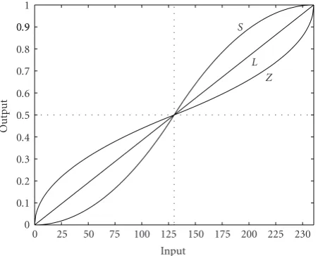
according to some criteria. Some of them are the Linear (L) function
μL
f;a,r= f −a
r−a, (12)
S-function
μS
f;a,b,r= ⎧ ⎪ ⎪ ⎪ ⎪ ⎪ ⎪ ⎨ ⎪ ⎪ ⎪ ⎪ ⎪ ⎪ ⎩ 2
f −a r−a
2
, a≤f ≤b,
1−2
f −r r−a
2
, b≤ f ≤r,
0 0.1 0.2 0.3 0.4 0.5 0.6 0.7 0.8 0.9 0.9 1
Output
0 25 50 75 100 125 150 175 200 225 230 Input
S
L Z
Figure1: Fuzzification functions:L,S,Zfunction.
and π-function [16, 17]. In signal representation, the fuzzification needed to be single valued and as such we will not consider theπ-function fuzzification. We propose a new fuzzification method, calledZ-function fuzzification, which has the inverse effect of theS-function fuzzification. TheZ -function is
μZ
f;a,b,r= ⎧ ⎪ ⎪ ⎪ ⎪ ⎪ ⎨ ⎪ ⎪ ⎪ ⎪ ⎪ ⎩
f −a
2(r−a), a≤ f ≤b,
1−
f −r
2(a−r), b≤ f ≤r,
(14)
whereμis the membership function and f,a,b, andr are the grey level, and the minimum, middle, and maximum value of the image grey level. Notice that these three functions are all single valued and monotonically increasing in the analysis interval (minimum to maximum of the signal). The fuzzification functions for image is shown in Figure 1. Given that the fuzzification functions chosen are single valued, the defuzzification process is easily achieved by the inverse mapping.
The application of these fuzzification techniques in signal analysis varies. For instance, the S-function enhances the image contrast about theblevel, and as such it could be used for edge enhancement. On the other hand, theZ-function decreases the contrast or blurs the image about theblevel. The linear fuzzification does not alter the contrast, it simply normalizes the image to a range of [0, 1].
To illustrate the application ofS-function in edge detec-tion, consider the fuzzy morphological gradient (FMG)
μd(n)=μf⊕k(n)−μfΘk(n) (15)
obtained as an extension of the classical morphological gradient first proposed by Serra [18] and Evans and Liu [19]. Applying the FMG to the real signal of an image in Figure 2(a), we obtain the lower figure where the peaks correspond to the edges. To enhance these edges, we con-sider the fuzzification of this result to achieve concon-siderable enhancement of the edges as shown inFigure 2(b).
3. Fuzzy Morphological Polynomial (FMP)
Representation
The FMP representation is analogous to the morphological polynomial transform [20] and the orthogonal polynomial representation [5]. Using fuzzy morphological opening we obtain a representation similar to a polynomial represen-tation by means of a geometrical decomposition of the signal. One of the difficulties encountered in the process was the selection of the structuring functions, which can be either arbitrary or derived from the signal. In our case, we get them from a complete set of ordered real-valued
orthogonal polynomials in 0 ≤ n ≤ N − 1. In the
examples, we use the discrete Legendre orthogonal (DLO) polynomials [21]. It should be noted that the corresponding membership functions are not necessarily orthogonal. Let
μf(n) be the membership function of a given signal, and μki(n) : 0≤i≤N−1}be one-dimensional fuzzy structuring
functions, such that 0 ≤ μki(n) ≤ 1. Let{ai} be adaptive
parameters used to make the fuzzy structuring function fit μf (n) closely. To consider all possibilities, the fuzzy
structuring functions{μki(n)}are derived from a shifted and
normalized set of orthogonal polynomials{μgi(n)}and its
complementary functions {μgc
i(n)}. Figure 3 illustrates the
shifted and normalized functions{μgi(n)}when we consider
the discrete Legendre orthogonal polynomials forN=5. The geometric decomposition of the given membership functionμf (n) is obtained recursively as follows.
(i) Windowing withW(n):
μvz0(n)=μf(n)×W(n−vN). (16)
(ii) Adaptive recursive approximation ofμz0(n):
μv
zi+1(n)=μ
v zi(n)−μ
v
zi◦aiki(n), (17)
wherei = 0, 1,. . .,N −1 relates to the structuring functionsaiμki(n),v=0, 1, 2,. . .refers to the window
W, andai are in [0, 1] adaptive parameter. Each
window is processed similarly.
The term a0μk0(n) is very important in the above
decomposition as it provides a coarse approximation to the signal membership function while{aiμki(n),i >0}gives the
fine information ofμv
z0(n). Applying (17) recursively we have
μvz0(n)=
N−1
i=0
μvzi◦aiki(n) +μ
v
zN(n), (18)
where the last term corresponds to the residual or the part of the signal that cannot be well represented withN function
μki(n). We will show in the next section that the above
representation can be considerably simplified by choosing values of{ai}such that
μvzi◦aiki(n)=aiμki(n) (19)
to convert (18) into
μv z0(n)=
N−1
i=0
0 0.1 0.2 0.3 0.4 0.5 0.6 0.7 0.8 0.9 1
M
ag
nitude
50 100 150 200 250 300 350 400 450 500
n
(a)
0 0.1 0.2 0.3 0.4 0.5 0.6 0.7 0.8 0.9 1
M
ag
nitude
50 100 150 200 250 300 350 400 450 500
n
(b)
Figure2: Effects ofS-function on edge enhancement (a) Original signal and edge detected, (b)S-function enhanced version (solid edges) of (b).
0 0.2 0.4 0.6 0.8 1
u
0 0.5 1 1.5 2 2.5 3 3.5 4
n
Figure3: Fuzzy structuring functions using DLO polynomials for
N=5.
representation analogous to a polynomial representation of the windowed signal.
Properties. The following propositions will give insight on how the FMP representation works and how to develop formulas to calculate the {ai} coefficients. Here, we work on a frame signal only, and thus the superscript v can be omitted. Also, we use min, max to stand for min0≤≤N−1
and max0≤≤N−1. In the following propositions, we assume μz(n),μk(n) are both defined on 0 ≤ n ≤ N −1, and {ai} ∈[0, 1] then
Proposition 1. The opening
μvzi◦aiki(n)=max 0,aiμki(n) +μc−1
, (21)
whereμc=1 + min{0, min[μzi()−aiμki()]}.
This proposition provides a simplification of the nonlin-ear opening and yieldμc, an index of the degree of fitting of
the structuring function in the signal membership function.
Proposition 2. There exists an optimum {ai} ∈ [0, 1] (denoted asa∗i ) such thatμvzi◦a∗iki(n)=a
∗
iμki,0≤n≤N−1,
if and only if the following optimum condition is satisfied
min
μzi()−a
∗ iμki()
=0. (22)
The valuea∗i is calculated as
a∗i = min 0≤l≤N−1
μki(l)=/0
μzi()
μki()
. (23)
LetJ(ai)=min[μzi()−aiμki()]be the fitting cost function,
and refer to
Ja∗i
=0 (24)
as theoptimumcondition. There are two direct corollaries that follow from this proposition.
Corollary 1. If the optimum condition is met, then, there are the following.
(i)Ifai> a∗i, thenJ(ai)<0,0≤n≤N−1,
(ii)Ifai< a∗i, thenJ(ai)>0,0≤n≤N−1,
(iii)a∗i =minn[μz0(n)].
(iv) 0≤a∗i ≤max[μzi(n)]≤1,0≤i≤N−1.
Corollary 2. If the optimum condition is met forμzc
0(n),then
a∗0c=maxn
μz0(n)
. (25)
Proposition 3. For μzi(n), i = 0, 1,. . .,N −1 in (17), the
following relation holds
(i) 0≤μzi+1(n)≤μzi(n)≤1,
(ii) minn[μzi+1(n)]=0.
This proposition shows that the residual at each decom-position step satisfies the membership function conditions, decreases, and at least in one point is zero.
Proposition 4. If the optimum condition is met foraiandai,
then the only value ofaiis zero to satisfy the following equations μzi◦aiki(n)=aiμki(n),μzi◦aiki(n)=a
iμki(n), for0≤i≤N−1,
whereμzi(n)μzi(n)−aiμki(n).
This proposition establishes that once geometrical fea-tures are decomposed from an input membership function, opening with previously used fuzzy structuring function gives zero.
3.1. Implementation. The representation ofμf(n) according
to (20) requires the calculation of the adaptive coefficient
{ai} and choosing the appropriate structuring functions. There are two possible methods to find the coefficients{ai}, the first one is based on a geometrically intuitive argument, while the second usesProposition 2given before. Consider a given window, and for simplicity let us not indicate it in the equation.
3.1.1. Calculation of{ai}
Iterative Method. Let aqi be the qth iteration of ai (a∗i as
theoptimum) when attempting to optimize the fitting cost function
J(ai)= min
0≤≤N−1 μzi()−aiμki()
, (26)
with respect toai, the optimum valuea∗i is obtained when
the cost is zero, and such thatμzi◦a∗iki(n)=a
∗ i μki(n).
According to (26) andCorollary 1, the following algo-rithm can be used to find the optimum value ofai:
a0i =max
μzi(n)
,
Jaqi
= min
0≤≤N−1 μzi()−a q i μki()
,
aq+1i =a q i +J
aqi
,
(27)
where q ≥ 0. That J(aqi) converges toward zero when q
increases can be established. If we assume thataqi > a∗i, then J(aqi)≤0 (Corollary 1), and, thus
Jaq+1i
= min
0≤≤N−1 μzi()−
aqi +J
aqi
μki()
≥ min
0≤≤N−1 μzi()−a q i μki()
=Jaqi
.
(28)
Direct Method. As in Proposition 2, we can compute
a∗i using (23). This method gives the samea∗i as the iterative
method, but in a faster way.
3.1.2. Choosing Structuring Functions. Given shifted and normalized orthogonal polynomials{μgi(n)}and their
com-plements{μgc
i(n)}, we need to determine which of these two
should be used as the structuring functions{μki(n)}for the
representation. This needs to be done due to the positivity condition on the adaptation coefficients{ai}. We decide this by comparing the reconstruction error corresponding to the coefficients attached to each of these structuring functions.
Let the coefficients ai and ai be the optimum values
forμgi(n) and μgic(n), respectively. We want to choose the
optimum value which gives us the smaller reconstruction error. Let the reconstruction error membership function corresponding toaiandaibe, respectively,
μe1(n)=μzi(n)−aiμgi(n),
μe2(n)=μzi(n)−aiμgc i(n).
(29)
It can be easily shown that
αi N−1
n=0
μgi(n)=
N−1
n=0 μgc
i(n), (30)
whereαiis found to be
αi= N−1N n=0 μgi(n)
−1 (31)
(noticeα0=0 and 1−μk0(n)=0, soi≥1). If
ai≤aiαi, (32)
then we have that
N−1
n=0
μe1(n)≥
N−1
n=0
μe2(n). (33)
In that case, we then letαi = ai andμki(n) = 1− μgi(n).
Otherwise, we chooseαi=aiandμki(n)= μgi(n).
4. Two-Dimensional Fuzzy Morphological
Polynomial Representation
The FMP representation can be easily generalized to two dimensions. Let μf(m,n) be the given signal membership
function and,μk∅(m,n), 0≤ ∅ ≤MN−1 be ordered two-dimensional fuzzy structuring functions, based on
orthogo-nal polynomials on 0 ≤m≤M−1, 0 ≤n≤N−1. The
geometrical decomposition algorithm becomes
μu,v
z0(m,n)=μf(m,n)×W(m−uM,n−vN),
μu,v
z∅+1(m,n)=μ
u,v
z∅(m,n)−μ
u,v
z∅◦a∅μk∅(m,n),
(34)
block is decomposed similarly. As in (18)–(20), our two-dimensional FMP representation for a frame signal is
μu,vz0(m,n)=
MN−1
∅=0
a∅μu,vk∅ (m,n) +μ
u,v
zMN(m,n). (35)
Notice that the ∅, abbreviation of ∅(i,j), is an order-ing function used for the two-dimensional structurorder-ing functions. The properties of one-dimensioned FMP can be extended to two dimensions easily, thus, we omit the
derivation here. As in the one dimension, the optimum
condition in the two dimensions is
min
s,t
μz∅(s,t)−a∗∅μk∅(s,t)
=0, (36)
wherea∗∅is an optimum value to satisfy this equation.
It is understood from the previous section that the one-dimensional algorithm can be extended to two-dimensional provided the generation and ordering of the two-dimensional structuring functions are determined. Sep-arable and nonsepSep-arable bivariate orthogonal polynomials may be used to generate two-dimensional structuring func-tions. Consider the separable structuring functions
μki,j(m,n)=μki(m)μkj(n) (37)
obtained from the one-dimensional structuring functions. Figure 4 shows an example of two-dimensional separable structuring functions with size of 5×5.
An inherent problem in two dimensions is the ordering of the structuring functions, which in the one-dimensional case occurs naturally. Our approach first investigates the structuring function properties and establishs the possible guides to the order of the two-dimensional structuring functions and then comes out a procedure to get the solution.
Proposition 5. If one multiplies two normalized one variate structuring functions, derived from the discrete Legendre orthogonal polynomials,μki(m)of sizeMandμkj(n)of sizeN
as two-dimensional structuring function, that is,μki,j(m,n)=
μki(m)μkj(n)with dimension ofM×N, then one can have the
following properties:
(i)μk0,j(m,n)≥μki,j(m,n)for alli,j,m,n.
(ii)μki,0(m,n)≥μki,j(m,n)for alli,j,m,n.
(iii)μk0,0(m,n)≥μki,j(m,n)for alli,j,m,n.
This proposition gives properties of the separable two-dimensional structuring functions based on one-dimensional DLO polynomials.
Proposition 6. If optimum condition is met for a∗∅(i,j) and a∗∅(s,t)and μk∅(i,j)(m,n) ≤ μk∅(s,t)(m,n)for a pair(i,j),(s,t)
and for allm,n, then the only value ofa∗∅(s,t)is zero to satisfy
the following equations:
μz∅(i,j)a∗∅(i,j)μk∅(i,j)(m,n)=a
∗
∅(i,j)μk∅(i,j)(m,n),
μz∅(s,t)a∗∅(s,t)μk∅(s,t)(m,n)=a
∗
∅(s,t)μk∅(s,t)(m,n),
(38)
where μz∅(s,t)(m,n) μz∅(i,j)(m,n)− a
∗
∅(i,j)μk∅(i,j)(m,n) − (m,n), with0≤(m,n)≤1, for allm,nand arbitrary such that0≤μz∅(s,t)(m,n)≤1.
This proposition gives guides of the structuring function order. If the structuring function has higher amplitude values than the other one at every point, then the structuring func-tion must have a lower order otherwise the decomposifunc-tion gets zero.
By observation, the factor in addition to the amplitude which affect the natural order of the one-dimensional struc-turing function is its complexity. Based on the properties and the observation, we come up with our rationale solution. We first define the amplitude and complexity index to quantitatively measure the structuring function amplitude and complexity characteristic.
Definition 1. An amplitude index (AI) of a geometrical structuring functionμki,j(m,n) of size M×N is defined by
the summation of amplitude at every pixel as
AIi,j= N−1
n=0 M−1
m=0
μki,j(m,n). (39)
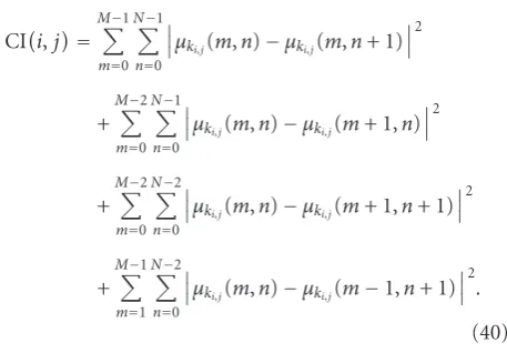
Definition 2. A complexity index (CI) of a geometrical structuring functionμki,j(m,n) of sizeM×N is defined by
the distance between the adjacent pixel in the horizontal, vertical, and diagonal directions as
CIi,j= M−1
m=0 N−1
n=0
μki,j(m,n)−μki,j(m,n+ 1)
2
+
M−2
m=0 N−1
n=0
μki,j(m,n)−μki,j(m+ 1,n)
2
+
M−2
m=0 N−2
n=0
μki,j(m,n)−μki,j(m+ 1,n+ 1)
2
+
M−1
m=1 N−2
n=0
μki,j(m,n)−μki,j(m−1,n+ 1)
2.
(40)
Based on the CI definition, the membership function is the simplest (constant) only if CI(i,j) = 0; if two fuzzy structuring functions have the same geometrical structures then they have the same complexity index CI(i,j) value.
Figure4: Two-dimensional separable structuring functions.
Definition 3. A structuring index (SI) of a structuring func-tionμki,j(m,n) with amplitude index AI(i,j) and complexity
index CI(i,j) is defined as
SIi,j=0.5 NAIi,j−1+NCIi,j, (41)
where 0.5 is average factor and N(·) is a normalization operator over the structuring functions.
Notice that the value of SI is in [0, 1].
Based on SI(i,j), the order of the fuzzy structuring functions is
∅i,j<∅(s,t),
iff SIi,j<SI(s,t),
or SIi,j=SI(s,t),
wheni < sori=s, j < t.
(42)
We can get the order of the two-dimensional fuzzy struc-turing functions from one variate DLO polynomials. As an example, this will order 5×5 two-dimensional structuring functions asTable 1. Our ordering method, considering both the amplitude and intrinsic geometrical complexity of the
Table1: Order of the structuring functionsμki,j(m,n) of size 5×5.
j
0 1 2 3 4
i
0 (0) (1) (4) (6) (16)
1 (2) (3) (8) (10) (8)
2 (5) (9) (12) (13) (20)
3 (7) (11) (14) (15) (22)
4 (17) (19) (21) (23) (24)
structuring function, is more reasonable than the commonly used close-neighbor ordering method [22], considering only the index of the structuring functions.
5. Applications
Table2: Signal to noise ratio (dB) for one-dimensional FMP.
L Z S
window sizes
3 4 5 3 4 5 3 4 5
1 25.53 23.43 21.84 25.53 23.43 21.84 25.53 23.43 21.84 2 32.72 28.59 26.04 32.46 28.43 25.93 32.71 28.58 26.01 3 34.60 29.57 27.09 33.37 29.16 26.65 33.74 29.17 26.16
4 30.07 27.55 29.67 27.20 29.71 26.52
5 27.95 27.56 26.56
5.1. Data Compression. The application of the FMP repre-sentation for data compression is shown in Figure 5. The signal f(n) is fuzzified byF and then processed by the FMP decomposition to get the adaptive coefficients. The signal membership function is reconstructed and f(n) is recovered by the defuzzifierD. The block diagram for two dimensional signals is similar. The pepper image with size of 512×512 shown inFigure 6is used as a test image.
In the first example, the one-dimensional FMP algorithm is used to process the test image horizontally. We consider different fuzzification methods, window lengths. The fuzzy structure functions are obtained from DLO polynomials as shown before. The performance of our representation is evaluated by the “peak-to-peak” signal to noise ratio (SNR dB) and the entropy-based compression ratio (ECR). The entropy-based compression ratio (ECR) is defined as
ECR= total l.c.of bits of compressed signal
total l.c.of bits of original signal = N−1
i=0 Mili MTlT
,
(43)
whereNis the number of subblock signals,Miis the number
of samples of the subblocki,liis the bits/sample required to
code subblocki,lTis the bits/sample required for the original
signal, MT is the total number of samples of the original
signal. The average bits/samplelirequired to code a subblock
signal is defined by entropy as
li= − G−1
j=0
pjlog2pj, (44)
where pj is a probability of a sample with amplitude j,G
is the greatest amplitude of the signal. In Table 2, signal-to-noise ratio (SNR dB) values for different fuzzification
methods and window sizes are shown. In Table 3, the
entropy-based compression ratio (ECR) for different fuzzi-fication methods and window sizes are shown. These results show that our one-dimensional algorithm has a high data compression when usingLorZfuzzification methods. The results also indicate that by using the Z fuzzification we achieve a higher compression ratio with good SNR than those results withLfuzzification.
In the second example, we apply our two-dimensional FMP algorithm to process block by block the test image. The fuzzy structuring functions are generated by multiplying two one-dimensional structuring functions derived from DLO
Table3: Compression ratio for one-dimensional FMP.
L Z S
window sizes
3 4 5 3 4 5 3 4 5
1 0.329 0.246 0.197 0.316 0.236 0.188 0.329 0.246 0.197 2 0.492 0.362 0.286 0.356 0.271 0.220 0.542 0.389 0.303 3 0.555 0.425 0.338 0.365 0.281 0.232 0.636 0.483 0.333
4 0.470 0.355 0.287 0.237 0.498 0.397
5 0.379 0.241 0.428
Table4: Signal to noise ratio (dB) for two-dimensional FMP.
L Z S
window sizes
3×3 4×4 5×5 3×3 4×4 5×5 3×3 4×4 5×5 1 22.41 20.29 18.73 22.41 20.29 18.73 22.41 20.29 18.73 2 24.54 21.89 20.69 24.56 21.91 20.66 24.49 21.84 20.67 3 27.80 24.15 21.89 27.75 24.13 21.86 27.68 24.01 21.82 ..
. ... ... ... ... ... ... ... ... ... All 29.01 26.12 23.05 28.89 25.04 22.66 28.79 25.91 22.57
Table5: Compression ratio for two-dimensional FMP.
L Z S
window sizes
3×3 4×4 5×5 3×3 4×4 5×5 3×3 4×4 5×5 1 0.109 0.061 0.039 0.104 0.058 0.037 0.109 0.061 0.039 2 0.160 0.088 0.057 0.115 0.065 0.043 0.178 0.095 0.061 3 0.199 0.109 0.069 0.123 0.071 0.046 0.230 0.123 0.076 ..
. ... ... ... ... ... ... ... ... ... All 0.281 0.163 0.119 0.128 0.075 0.050 0.370 0.207 0.152
polynomials. The order is determined by the structuring index method discussed before. In Table 4, we show the signal-to-noise ratio (SNR dB) for different fuzzification methods and window sizes. In Table 5, the entropy-based compression ratio (ECR) for different fuzzification methods and window sizes is shown. Those results indicate that our two-dimensional algorithm has a higher performance when usingLandZfuzzification methods. The results also indicate that theZfuzzification achieves a higher compression ratio with good SNR than the L fuzzification. To illustrate the results, we show in Figures7(a)and7(c) and Figures7(b) and7(d)the FMP component and the corresponding error images, when using window size of 1×3 and 3×3, forL -function fuzzification.
Since there is no published papers, as we know, using the fuzzy morphology approach for data compression, we want to show the high performance of our algorithm by comparing with those obtained by commonly used high performance method such as discrete cosine transform (DCT) [23]. In order to have a fair comparison, we use
the coefficients with high energy of the DCT and FMP
f(n)
F
μv z0(n)
μv z1(n)
+ −
+ −
a0μk0(n)
a1μk1(n)
μvf0(n)
μv f1(n)
a0
a1
μk0(n)
μk1(n)
μvz0(n)
D
f(n) +
Figure5: FMP representation block diagram.
Figure6: Original Image for analysis.
Table6: Comparison for one-dimensional FMP and DCT.
FMPZ DCT
3 4 5 3 4 5
SNR (dB) 32.46 29.67 27.56 32.31 29.54 27.40
ECR 0.356 0.287 0.241 0.415 0.312 0.262
image which is closely used in [26,27], then we compare their data compression ratio at each different window size. The comparisons of SNR (dB) and ECR are shown in Tables 6 and 7 for one and two dimension, respectively. Those results indicate that our FMP representation usingZ fuzzification achieves the higher data compression ratio that of DCT. We also provide, as an example, the one- and two-dimensional reconstructed images inFigure 8using the FMP representation with Z fuzzification and the DCT method, with window size of 3 and 3×3 cases, for visual quality comparison purpose.
Figures 8(a)and8(c) and Figures 8(b)and 8(d)show the reconstructed images for one and two dimensions, respectively. Figures 8(a)and 8(b)show the reconstructed images using FMP with Z fuzzification. Figures 8(c) and 8(d)show the the reconstructed images using DCT. Those
Table7: Comparison for two-dimensional FMP and DCT.
FMPZ DCT
3×3 4×4 5×5 3×3 4×4 5×5 SNR (dB) 28.89 25.04 22.66 28.70 24.89 22.54
ECR 0.128 0.075 0.050 0.147 0.092 0.061
Table8: Computation Complexity of FMP and DCT.
Operation FMP DCT
Mul./Div. N2 3N2+ 3N
Add./Sub. 4N 2N2−N
Min./Max. N2+ 2N —
Lut/Chk N2−N N2
Total 3N2+ 5N 6N2+ 2N
results indicate that the visual quality of using our FMP representation withZfuzzification and DCT method is sim-ilar. However, our FMP representation withZfuzzification achieves higher data compression ratio (fewer bits/pixel). For computation complexity comparison,Table 8shows the required operations including addition/subtraction, multi-plication/division, and minimum/maximum and look-up table/check-up for FMP and DCT. Assume a window size of N is used. Notice that the multiplication/division and addition/subtraction operations contribute more computa-tion complexity than the other operacomputa-tions. We can see clearly that the FMP requires less number of operations than that of the DCT.
(a) (b)
(c) (d)
Figure7: One- and two-dimensional FMP representation: (a) and (c) one-dimensional FMP component and error images, respectively, (b) and (d) two-dimensional FMP components and error image, respectively.
5.2.1. One-Dimensional Estimation. Let μf(n), 0 ≤ n ≤ M−1, be the membership function of a signal f(n). For each of the signal frames, we will use {μki(n)}, 0 ≤ n ≤
[0,N−1], as structuring functions based on the discrete
Legendre polynomials (see Figure 3 when N = 5). The
FMP algorithm provides the adaptation parameters{ai}, for each frame membership functionμz(n).Let then the support
length of μf(n) be S = M−1 (if we know the sampling
period Ts thenS = (M−1)Ts) which is divided into an
integer number of windows of increasing lengthr =N−1 (orr=(N−1)TswhenTsis known).
For each of the frames, we will attempt to come up with a cover that encloses the signal as tightly as possible. The length of the cover can be calculated recursively from the FMP adaptive coefficients and the values of the structuring functions. For a frame v with corresponding length r, we have that (SeeFigure 9whenr=4)
0v(r)= r S,
iv(r)= r
j=1
μki
j−μki
j−12avi 2
+
iv−1(r) r
2
,
(45)
where 0v(r) is the geometric length corresponding to the
constant FMP decomposition, and i = 1, 2,. . .,I, I ≤
r corresponds to the ith FMP geometric decomposition.
j = 1, 2,. . .,r corresponds to the point of the structuring function. The length calculation is done in each of the r
segments in which the window is divided (SeeFigure 9). The height of the the coverdv(r)∈[0, 1] can be found exactly in
the case whereμv
z(n) is either a constant or has a great deal
of variation. In the first case,dv(r)=0, and in the second, dv(r) = 1. However, it should be noted that in these two
cases, we will have avi = 0,i > 0 that is only a constant
approximation is possible. In cases different from the above ones, we cannot calculate dv(r) exactly although a good
estimate of it can be obtained as the difference between the
maximum and minimum of the residualμv
zI+1(n) (see (18)) obtained after theIth decomposition. Thus, the diagonal of the cover in framev
v(r)=v I(r)
2
+ (dv(r))2 (46)
can be used as an estimate of the length of the signal for that correspondingr.
Summing up the number of instruments contributions for eachr,
Q(r)= [S/r]
v=1 v(r) v0(r)
(a) (b)
(c) (d)
Figure8: Reconstruction images: (a) and (c) for one-dimensional FMPZfuzzification and DCT method, respectively, (b) and (d) for two-dimensional FMPZfuzzification and DCT method, respectively.
1 2 3 4
ν
l1
a1
a0 l0
Figure9: Frame signal length approximation.
Using least-square fitting in the log(Q(r)) versus log(1/r) graph for various values of r, the slope of the line will correspond to an estimate of the FD.
Remarks. (1) In order for the above discrete algorithm to work properly, we need to chooser so thatS/ris an integer for every chosen value ofr. Results vary for different choices ofrdue to the global linear fitting. A better estimate might be
obtained by doing the the linear fitting piecewise, obtaining a better estimate for linear fitting for smallrs.
(2) If μf(n) is so smooth that the FMP givesavi = 0,
0 < i ≤ I, for everyv, then we have that dv(r) ≈ 0, and v(r)/v
0(r)=1 and, therefore,Q(r)=S/rfor any value ofr.
The estimation of the slope of log(Q(r)) versus log(1/r) for two different values ofrgives that the fractal dimensionDis one.
(3) On the other hand, ifμf(n) varies widely everywhere,
then the FMP givesavi =0, 0≤i≤I, for everyv, but due to
the large variationdv(r)≈1, in which casev
I(r)=v0(r). We
will then get that
v(r) v
0(r) =
1 +S
2
r2 ≈ S
r, (48)
after substituting dv(r) and v
0(r), and using the fact that S/r 1 (i.e., we divideSinto several windows) which will give usQ(r) = S2/r2, so that the slope estimation for two
D=1.2
D=1.5
D=1.8
Figure10: WCF generated signals with different FD.
Table9: Estimated FD of WCF signal.
True D 1.2 1.3 1.4 1.5 1.6 1.7 1.8
Our D 1.237 1.271 1.358 1.505 1.648 1.721 1.825 MC D 1.227 1.327 1.424 1.515 1.606 1.701 1.797
(5) Due to the significance of the constant of the FMP approximation, a very efficient algorithm can be found when only that component is considered. We then have that
v(r)=v 0(r)
2
+ (dv(r))2,
Q(r)= [S/r]
v=1
!1 +dv(r) v
0(r) 2
,
(49)
from which estimation of the FD can be done as before. To test our algorithm, artificial fractal signals with known FD are generated using the weistrass cosine function (WCF) method [24, 28]. Figure 10 shows some WCF generated signals, and when we apply our procedure to them. The results are shown in Table 9. For comparison purpose, the results of using MC method [24] are also shown in the table.
5.2.2. Two-Dimensional Estimation. Different from the one-dimensional case, the estimation of the FD of a two-dimensional signal can only be done using the constant and linear term of the FMP approximation. Using just the first three terms of the approximation, we have for anr×rblock of a square image of dimensionS×Sthat get the following recursive formulas:
Au,v0 (r)=
r S
2
,
Au,vi (r)=
au,vi 2
Au,vi−1(r) +
Au,vi−1(r) 2
,
(50)
where {au,vi } are coefficients found using the FMP. Notice
that these equations are similar to those in the one-dimensional case, except that in this case the block is not subdivided as we did with the window in the one-dimensional case. A cube covering the signal can be thought of having a base with areaAu,vI (r) and an approximate height
ofdu,v(r) equal to the difference between the maximum and
the minimum ofμu,v
z (n). The diagonal plane of this cube has
an area equal to
Au,v(r)=Au,v I (r)
2
+Au,vI (r)(du,v(r)) 2
, (51)
a formulation analogous to that in the one-dimensional case, when we use only two components
Q(r)= u,v
Au,v(r) Au,v0
. (52)
Similar comments as those made in the one-dimensional case can be made here. As before,S/rmust be an integer and the FD varies for different choices ofr. Likewise a very smooth signal has an FD close to 2, and a very rough signal has an FD close to 3.
Finally if in the FMP approximation we only use thea0
component, the above algorithm simplifies to
Au,v0 (r)=
r S
2
,
Au,v(r)=Au,v0 (r) 2
+Au,v0 (r)(du,v(r))2,
Q(r)= u,v
!1 +(du,v(r))2 Au,v0
,
(53)
from which we can find an estimate of the FD of the given two-dimensional signal.
We then apply our algorithm to estimate the FD of the Brodatz texture images [29] shown inFigure 11. The code of texture image is same as in the Brodatz album. The results are shown inTable 10. This example shows the applicability of our algorithm to estimate FD to images. We also show the results of using DBC method [25] for comparison purpose. The results of using these two methods are similar.
6. Conclusion
D03 D04 D05 D09
D24 D28 D33 D54
D25 D68 D84 D92
Figure11: Texture images.
Table10: Estimated FD of texture images.
D03 D04 D05 D09 D24 D28 D33 D54 D55 D68 D84 D92
Our D 2.55 2.69 2.49 2.67 2.54 2.64 2.51 2.46 2.60 2.7 2.72 2.64
DBC D 2.60 2.66 2.54 2.59 2.54 2.55 2.23 2.39 2.48 2.52 2.60 2.50
of the Pitas and Venetsanopoulos [8–10] and of Song and Delp [11] on morphological signal representation. We have applied our representation to data compression and fractal dimension estimation for one- and two-dimensional signals, the experimental results have shown the high performance in data compression and applicability in estimating fractal dimension as compared with those using the DCT [23], MC [24], and DBC [25] methods.
Appendix
Proof ofProposition 1.By definition
μzi◦aiki =μ(ziΘaiki)⊕aiki. (A.1)
According to fuzzy morphological erosion
μziΘaiki(n)=min
,n+
min1, 1−aiμki() +μzi(n+)
=min
min1, 1−aiμki() +μzi()
=μcδ(n).
(A.2)
Now
μc⊕aiki(n)=max
,n−
max 0,aiμki() +μcδ(n−)−1
=max 0,aiμki(n) +μc−1
.
(A.3)
Proof ofProposition 2.FromProposition 1,
μzi◦aiki(n)=
⎧ ⎨ ⎩
aiμki(n) +μc−1, aiμki(n) +μc−1≥0,
0, aiμki(n) +μc−1<0,
(A.4)
One wantμzi◦aiki(n)=aiμki(n).Sinceaiμki(n)≥0, for alln,
then a sufficient condition for this to happen is to set
μc = 1. From Proposition 1, one can have μc = 1 +
min{0, min[μzi()−aiμki()]}. That μc = 1 means that
min{0, min[μzi()−aiμki()]} =0, which implies that
min
μzi()−aiμki()
≥0. (A.5)
The optimum (maximum) value of ai (denoted as a∗i)
satisfying (A.5) is reached when the equality holds.
(1) Existence ofa∗i.
By contradiction, assume for allai∈[0, 1] such that
min[μzi()−aiμki()]=/0.There are two cases:
(a) min[μzi() − aiμki()] > 0. ⇒ μzi() >
aiμki() for all, which is not true, in particular
whenai=1 andμki()=1 for some.
(b) when min[μzi()−aiμki()] < 0 is similarly
shown.
(2) Uniqueness ofa∗i.
min[μzi()−aiμki()]=0⇒
μzi()≥aiμki(), ∀. (A.6)
Ifμki()=0, for some ∈[0,N−1], then (A.6) is
always satisfied, so one needs to consider only when
μki()>0, for whichai≤μzi()/μki(), Therefore,
a∗i = min 0≤≤N−1
μki()=/0
μzi()
μki()
. (A.7)
Proof ofCorollary 1. (i) It follows fromProposition 2. Ifai> a∗i , then
μzi()−aiμki()< μzi()−a
∗
i μki(), (A.8)
taking minimum over, we getJ(ai)< J(a∗i)=0.
(ii) Ifai< a∗i can be similarly shown.
(iii) ByProposition 2andμk0(n)=1.
(iv) By the antiextensive property of opening and optimum conditionμzi◦a∗iki(n)=a
∗
iμki(n)≤μzi(n).
By Proposition 1μzi◦a∗iki(n) ≥ 0 ⇒ 0≤a
∗
iμki(n) ≤
μzi(n).Thus, 0≤a
∗
imaxn[μki(n)] ≤ maxn[μzi(n)] ≤ 1, and
0≤a∗i ≤maxn[μzi(n)]≤1.
Proof ofCorollary 2. ByProposition 2andμk0(n)=1.a∗0 =
minn[μzc
0(n)].Thus,a
∗c
0 =maxn[μz0(n)].
Proof ofProposition 3.(i) According to the antiextensive property of opening μzi◦aiki(n) ≤ μzi(n) then μzi+1(n) =
μzi(n)−μzi◦aiki(n)≥0, soμzi+1(n)≤μzi(n).
(ii) By (17) andProposition 2, we get
min
n
μzi+1(n)
=min
n
μzi(n)−μzi◦aiki(n)
=0. (A.9)
Proof ofProposition 4.This can be proven easily using (22) and (23).
Proof ofProposition 5.By definition,
μki,j(m,n)=μki(m)μkj(n). (A.10)
We have
μk0,j(m,n)=μk0(m)μkj(n)
≥μki(m)μkj(n), ∀m,n,i,j.
(A.11)
Notice thatμk0()≥μki(), for alli,.
(ii) and (iii) are similarly shown.
Proof ofProposition 6.By optimum condition,
μz∅(s,t)a∗∅(s,t)μk∅(s,t)(m,n)=a
∗
∅(s,t)μk∅(s,t)(m,n)
a∗φ(s,t)
= min
p,q μkφ(s,t)(p,q)=/0
μzφ(s,t)
p,q μkφ(s,t)
p,q
≥0
= min
p,q μkφ(s,t)(p,q)=/0
μzφ(i,j)
p,q−a∗φ(i,j)μkφ(i,j)
p,q− ∈p,q μkφ(s,t)
p,q
≤ min
p,q μkφ(s,t)(p,q)=/0
μzφ(i,j)
p,q−a∗φ(i,j)μkφ(i,j)
p,q μkφ(s,t)
p,q
≤ min
p,q μkφ(i,j)(p,q)=/0
μzφ(i,j)
p,q−a∗φ(i,j)μkφ(i,j)
p,q μkφ(i,j)
p,q
=a∗φ(i,j)−a∗φ(i,j)
=0.
(A.12)
Therefore,a∗φ(s,t)=0.
References
[1] J.-L. Starck, M. Elad, and D. L. Donoho, “Image decompo-sition via the combination of sparse representations and a variational approach,”IEEE Transactions on Image Processing, vol. 14, no. 10, pp. 1570–1582, 2005.
[3] S. G. Mallat, “Theory for multiresolution signal decomposi-tion: the wavelet representation,”IEEE Transactions on Pattern Analysis and Machine Intelligence, vol. 11, no. 7, pp. 674–693, 1989.
[4] S. G. Mallat, “Multifrequency channel decompositions of images and wavelet models,”IEEE Transactions on Acoustics, Speech, and Signal Processing, vol. 37, no. 12, pp. 2091–2110, 1989.
[5] J. Martens, “The Hermite transform—theory,”IEEE Transac-tions on Acoustics, Speech, and Signal Processing, vol. 38, no. 9, pp. 1595–1606, 1990.
[6] J. Martens, “The Hermite transform—applications,” IEEE Transactions on Acoustics, Speech, and Signal Processing, vol. 38, no. 9, pp. 1607–1618, 1990.
[7] D. Shinha and E. R. Dougherty, “Fuzzy mathematical mor-phology,”Journel of Visual Communication and Image Process-ing, pp. 286–302, 1992.
[8] I. Pitas and A. N. Venetsanopoulos, “Morphological shape decomposition,” IEEE Transactions on Pattern Analysis and Machine Intelligence, vol. 12, no. 1, pp. 38–45, 1990.
[9] I. Pitas, “Morphological signal decomposition,” inProceedings of the International Conference on Acoustics, Speech, and Signal Processing (ASSP ’90), pp. 2169–2172, Albuquerque, NM, USA, April 1990.
[10] I. Pitas and A. N. Venetsanopoulos, “Morphological shape representation,” inProceedings of the International Conference on Acoustics, Speech, and Signal Processing (ICASSP ’91), pp. 2381–2384, Toronto, Canada, May 1991.
[11] J. Song and E. J. Delp, “The analysis of morphological filters with multiple structuring elements,”Computer Vision, Graphics and Image Processing, vol. 50, no. 3, pp. 308–328, 1990.
[12] C. Huang and L. F. Chaparro, “Signal representation using fuzzy morphology,” in Proceedings of the 3rd International Symposium on Uncertainty Modeling and Analysis and Annual Conference of the North American Fuzzy Information Processing Society, (ISUMA-NAFIPS ’95), pp. 607–612, IEEE, September 1995.
[13] G. Matheron,Random Sets and Integral Geometry, Wiely, New York, NY, USA, 1973.
[14] L. A. Zadeh, “Fuzzy sets,”Information and Control, vol. 8, no. 3, pp. 338–353, 1965.
[15] D. Dubois and H. Prade,Fuzzy Sets and Systems Theory and Applications, Academic Press, New York, NY, USA, 1980. [16] H. Bandemer and W. Nather, Fuzzy Data Analysis, Kluwer
Academic Publishers, Dordrecht, The Netherlands, 1992. [17] L. A. Zadeh, K. S. Fu, K. Tanaka, and M. Shimura, Fuzzy
Sets and Their Applications to Cognitive and Decision Processes, Academic Press, New York, NY, USA, 1975.
[18] J. Serra,Image Analysis and Mathematical Morphology, Aca-demic Press, New York, NY, USA, 1982.
[19] A. N. Evans and X. U. Liu, “A morphological gradient approach to color edge detection,”IEEE Transactions on Image Processing, vol. 15, no. 6, pp. 1454–1463, 2006.
[20] H. Cha and L. F. Chaparro, “A morphological polynomial transform,” inProceedings of the International Conference on Acoustics, Speech, and Signal Processing (ICASSP ’93), vol. 5, pp. 173–176, April 1993.
[21] C. P. Neuman and D. I. Schonbach, “Discrete (legendre) orthogonal polynomials—a survey,”International Journal for Numerical Methods in Engineering, vol. 8, pp. 743–770, 1974.
[22] L. F. Chaparro and M. Boudaoud, “Two-dimensional linear prediction covariance method and its recursive solution,”IEEE Transactions on Systems, Man and Cybernetics, vol. 17, no. 4, pp. 617–621, 1987.
[23] R. Gonzales and R. E. Woods, Digital Image Processing, Prentice-Hall, Englewood Cliffs, NJ, USA, 3rd edition, 2008. [24] P. Maragos and F. Sun, “Measuring the fractal dimension
of signals: morphological covers and iterative optimization,” IEEE Transactions on Signal Processing, vol. 41, no. 1, pp. 108– 121, 1993.
[25] N. Sarkar and B. B. Chauduri, “Efficient differential box-counting approach to compute fractal dimension of image,” IEEE Transactions on Systems, Man and Cybernetics, vol. 24, no. 1, pp. 115–120, 1994.
[26] S.-H. Jung, S. K. Mitra, and D. Mukherjee, “Subband DCT: definition, analysis, and applications,”IEEE Transactions on Circuits and Systems for Video Technology, vol. 6, no. 3, pp. 273–286, 1996.
[27] B. Kosko,Neural Network and Fuzzy System, Prentice-Hall, Englewood Cliffs, NJ, USA, 1991.
[28] B. B. Mandelbrot, The Fractal Geometry of Nature, W. H. Freeman, San Francisco, Calif, USA, 1982.