Theories in Laboratory and Field Experiments.
Thesis by
Debajyoti Ray
In Partial Fulfillment of the Requirements
for the Degree of
Doctor of Philosophy
California Institute of Technology
Pasadena, California
2015
Contents
Abstract ix
1 Introduction 1
1.1 Behavioural Economics . . . 2
1.2 Experimental Economics . . . 8
1.2.1 Errors in Lab Experiments . . . 10
1.2.2 Field Experiments . . . 12
1.3 Methods . . . 13
1.3.1 Submodularity and Greedy Algorithms . . . 13
1.3.2 Discrete Choice models . . . 16
1.4 Findings and Contributions . . . 18
2 Bayesian Rapid Optimal Adaptive Designs 20 2.1 A brief history of related adaptive methods . . . 23
2.2 Models . . . 25
2.3 Dynamic Optimal Designs . . . 29
2.3.1 Bayesian Active Learning in the Noiseless Case . . . 30
2.3.2 The Equivalence Class Determination Problem . . . 32
2.3.3 Noisy Observations . . . 35
2.3.4 A simple illustration . . . 37
2.4 Implementation: Efficiency and Challenges . . . 40
2.4.1 Effective Implementation . . . 40
2.4.2 Accelerated Greedy Evaluation . . . 41
2.5 Design and Evaluation . . . 43
2.5.1 Ground Truth Analyses . . . 43
2.6 Manipulation . . . 48
2.6.1 Noise Specification . . . 51
2.7 Empirical Data and Analysis . . . 53
2.7.2 Interpretation of Results . . . 55
2.8 Conclusions and future directions . . . 58
3 Time Preference 70 3.1 Models . . . 74
3.2 Optimal Adaptive Design . . . 76
3.2.1 A brief history of related adaptive methods . . . 76
3.2.2 A simple illustration . . . 78
3.2.3 Bayesian Active Learning in the Noiseless Case . . . 79
3.2.4 The Equivalence Class Determination Problem . . . 81
3.2.5 Noisy Observations . . . 82
3.3 Implementation . . . 84
3.3.1 Experimental Setup . . . 84
3.3.2 Ground Truth Analysis . . . 84
3.4 Analysis . . . 88
3.4.1 Hyper-patience . . . 90
3.4.2 Distribution of Parameters . . . 91
3.5 Discussion . . . 93
3.6 Instructions . . . 94
3.7 Subjective Time . . . 95
3.7.1 Simulations . . . 97
3.7.2 Discussion . . . 99
4 Reference Dependence and Substitution 106 4.1 Dataset . . . 108
4.2 Motivating Analysis . . . 109
4.2.1 Behaviour of Experienced Consumers . . . 112
4.3 Structural Model . . . 113
4.3.1 Estimation . . . 114
4.3.2 Identification . . . 115
4.4 Results . . . 116
4.4.1 Simulations . . . 116
4.4.2 Estimation from Retail Data . . . 118
4.4.3 Effect of Experience . . . 120
5 Discussions 124
5.1 Future Directions . . . 125
5.1.1 New measurements in Experimental design . . . 125
5.1.2 Applications of BROAD . . . 128
List of Figures
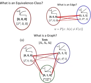
2.1 Constructing Equivalence Class Graphs. (top left) An equivalence class is the set of hypotheses
that generate the same vector of outcomes. (top right) An edge joins two observation vectors
generated by hypotheses from a sequence of tests in distinct equivalence classes. (bottom) An
EC2graph consists of all equivalence classes and the edges connecting them. . . . . 38
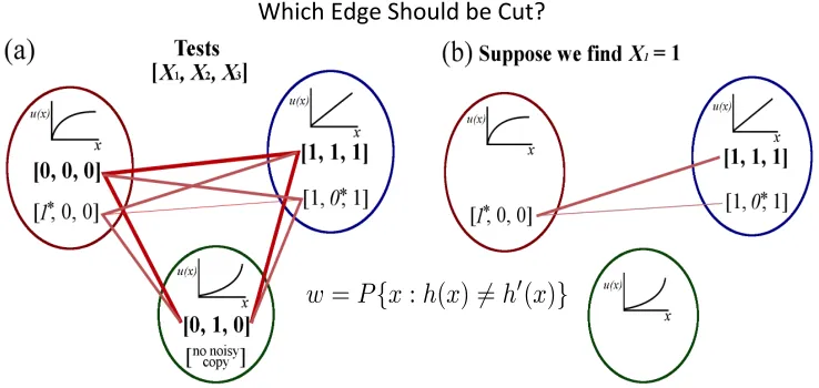
2.2 A stylized example of Equivalence Class Edge Cutting. . . 39
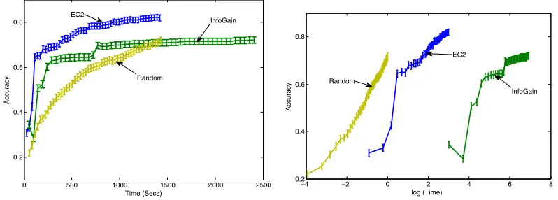
2.3 (Left) Accuracy as a function of time assuming a response time of 28 seconds (average response
time across all subjects). (Right) Accuracy as a function of logarithmic time with no response
delay. . . 42
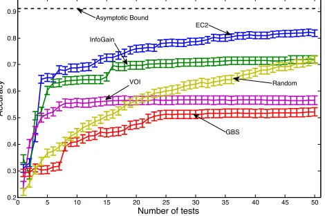
2.4 Performance of the algorithms when probability of error,= 0.05. The asymptotic bound from running all tests in random order is also shown. . . 45
2.5 Performance of the algorithms when probability of error,= 0.10. The asymptotic bound from running all tests in random order is also shown. . . 45
2.6 Performance of the algorithms when probability of error,= 0.20. The asymptotic bound from running all tests in random order is also shown. . . 46
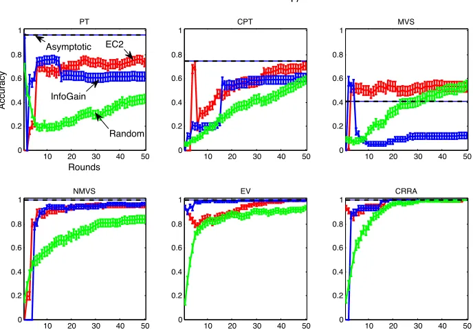
2.7 Performance of the algorithms for individual models when probability of error,= 0.05. The asymptotic bounds are also shown for recovering individual models. . . 47
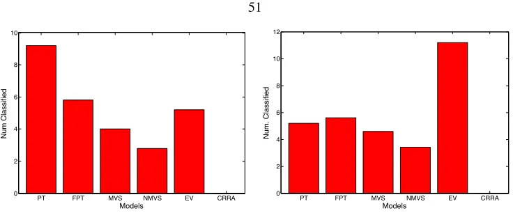
2.8 The classifications for the two treatments to test for manipulability. Treatment 1 has 27 subjects,
and treatment 2 has 30 subjects. The difference between the two distributions was not found to
be statistically significant. . . 51
2.9 Stacked bar plot of posterior distribution over the 6 models (averaged over the final 5 rounds)
for 27 subjects in the non-manipulation condition (left) and the manipulation condition (right). 51
2.10 Performance of the algorithms for individual models when probability of error,σ= 0.86for an average error rate of 10%(left) andσ= 1.12for an average error rate of 20% (right). . . 52 2.11 Examples of the dynamically-estimated posterior probability over all models for two subjects.
The subject on the left is rapidly classified as EV; the one on the right is less rapidly classified
2.12 Stacked bar plot of posterior distribution over the 6 models (averaged over the final 5 rounds)
for 57 subjects. The subjects are ordered on the x-axis based on maximum posterior probability
into models EV, FPT, CPT, MVS, SMVS and CRRA . . . 54
2.13 The posterior distribution of the 6 models after each round. The aggregate mean and standard
error is shown for 57 subjects. . . 55
2.14 The percentage of subjects whose current classification in a round, corresponds to final
classifi-cation (in round 30). Subjects trying to manipulate the algorithm might misrepresent their true
type in early rounds. . . 55
2.15 (left) A cartoon of the hypothetical reaction times in the two treatments to test for manipulation.
We expect higher reaction times when subjects are trying to manipulate. (right) The actual
reaction times with standard error bars for the two treatments. . . 56
2.16 The “collapsed” classification of 57 subjects into the four class of theories: Prospect Theory
(PT), Moments Models (MVS), Expected Value (EV) and Constant Relative Risk Aversion
(CRRA). . . 56
2.17 Sorted values of tests for the acceleratedEC2implementation. . . 64
3.1 A stylized example of Equivalence Class Edge Cutting. . . 76
3.2 The posterior distribution of the 5 models after each round. The aggregate mean and standard
error is shown for 40 subjects. . . 89
3.3 The classification of 40 subjects to each of the 5 models. . . 89
3.4 The posterior distribution of the 5 models after each round. The aggregate mean and standard
error is shown for 40 subjects. . . 90
3.5 The classification of 40 subjects to each of the 5 models with expanded parameter support for
“hyper-patience”. . . 91
3.6 The calendar time and biological time evolve at different rates. Two equal intervals(0,∆)
and(s, s+ ∆)in calendar time (horizontal axis) translate into unequal intervals(t0, t∆)and (ts, ts+∆)in biological time (vertical axis). The functionF(·)depicts one possible realization
of the (stochastic) transformation from calendar to biological time. . . 99
3.7 (Top) No autocorrelation of biological time (ρ= 0). The discounting curve in biological time is exponential with discount rate equal to 1. It generates the dotted discounting curve in calendar
time (“ZeroCorr”). The best exponential (“Exp”) fit in calendar time produces a discount rate
of 0.30, and the best hyperbolic fit (“Hyp”) has a discount rate equal to 2.75. (Bottom) Very
high autocorrelation of biological time (ρ= 0.97). The discounting curve in biological time is exponential with discount rate equal to 1. It generates the dotted discounting curve in calendar
time (“HighCorr”). The best exponential (“Exp”) fit in calendar time produces a discount rate
3.8 Impact of increased variability onto shape of discounting under mild autocorrelation of the
biological clock (ρ= 0.3). As variability (“Var”) increased from 0.5 over 1 to 4, the discounting function becomes more convex. . . 104
3.9 Time intervals generated from concavity in the mapping from calendar to biological time,
induced by decreasing the speed of the biological clock for time intervals further into the future
(γ= 0.5). The biological clock does not exhibit autocorrelation (ρ= 0). The discounting curve in biological time is exponential with discount rate equal to 1. The dashed-dotted line depicts
the resulting discounting curve in calendar time (“Concav”). The best exponential (“Exp”) fit
in calendar time produces a discount rate of 0.40, and the best hyperbolic fit (“Hyp”) has a
discount rate equal to 2.20. . . 105
4.1 Simulated effect of loss aversion and substitution with each point a different sample of loss aversion parameterλ(sampled uniformly between 1 and 4). When higher selling item (black dots), goes on sale (periods indicated by blue line), quantity increases. When sale ends, the quantities sold decrease whilst, due to loss aversion, the relative utility of a lower selling substitute (red dots) increases. At each period the loss aversion parameter is sampled from a distribution. . . 107 4.2 A snapshot of the retailer’s website powerdrills. Consumers can easily look at the price of the item of
interest, whether it is currently at a discount, as well as the price and discount status of substitutes. . . . 109 4.3 The total sales, in log scale, of all 6039 SKUs ranked (left). The total sales made by customers in log scale,
in ranked order (right). . . 110 4.4 The total amount of discounts offered per day over 19.5 months (left). The fraction of days the items
(ordered according to sales rank) are on sale in the last 8 months (right). . . 111 4.5 (left) The effect of Discounts (day 0) and days since the last discount period for the top 1000 SKUs. (right)
The effect for “experienced” customers (red line) and “inexperienced” customers (black line). . . 112 4.6 The $100 gift card has a spurt in sales during sale periods (indicated by black dots). Once the sale is
removed, the quantities sold decline whilst the substitute, $50 gift card, has a greater increase in sales. On the right: The effect on sales since the day the last sale ended (black line). A sale ending for the substitute (red line) has a positive effect on the substitute. The quantities and discount periods are smoothed using a 5-day window. . . 113 4.7 The probability of choosing first item,P(Ci= 1), for no loss aversion,λ= 1on left.P(Ci= 1)for
loss aversion coefficientλ= 3on right. . . 117 4.8 A histogram of the estimated values ofλfor all 3673 substitute pairs. . . 119 4.9 The estimates ofλ(and errorbars) for substitute and non-substitute goods among the general (left),
experienced(middle) andinexperiencedcustomers (right). . . 121
5.1 Response times (in milliseconds) in choosing between two delayed rewards in Risky Choice
List of Tables
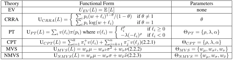
2.1 We compare 6 models of risky choice, with no parameters: Expected Value (EV), one parameter:
Constant Relative Risk Aversion (CRRA), adn 3 parameters: Prospect Theory (PT), Cumulative
Prospect Theory (CPT), Mean-Variance-Skewness (MVS), Normalized Mean-Variance-Skewness 25
2.2 Summary of the experimental design methods that are compared against EC2 . . . 43
2.3 Misclassification Matrix: Percentage of samples (row) that are classified as another model
(column) using EC2 after 50 rounds. The diagonal represents correct classification. . . 46
2.4 Differences in Misclassification Matrix: Percentage of samples (row) that are classified as
another model (column) using EC2 after 50 rounds fornoise minus the Softmax noise model
for average error rate of 0.10. The diagonal represents no difference in classification accuracy. 52
2.5 The User Interface presented to the participants. The two amounts and probabilities for the 2
lotteries are shown in text on the right. The same information is displayed as a graph on the left. 60
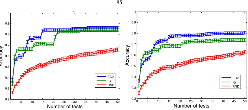
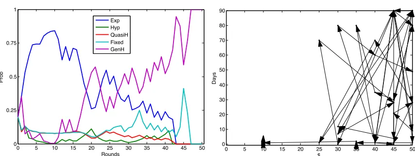
3.1 Performance of the algorithms when there is no error,= 0.0(left) and when probability of error,= 0.05(right). . . 85 3.2 Performance of the algorithms when probability of error,= 0.10(left) and= 0.20(right). . 85 3.3 The posterior probability of the models over 50 rounds for a ”Hyperbolic” type (left) and the
choice path: amount and delay of the options selected (right). . . 88
3.4 The posterior probability of the models over 50 rounds for a ”General-Hyperbolic” type (left)
and the choice path: amount and delay of the options selected (right). . . 88
4.1 Examples ofλvalues for 3 top-selling SKUs along with their substitute SKUs as well as examples of non-substitute SKUs. The ratio of the log-Likelihood of the pair under the multinomial choice model for the MLEλvalue, and forλ= 1is also shown; logRatio= logL(λ
∗
)
Acknowledgements
When I started my doctoral program, I was motivated to find the right answers upon completing my thesis. I
naively believed that somehow I’d devise methods to query human nature and find interesting answers. As I
write my thesis, I realize I have so many more questions to ask and very few right answers. What I have gained
during my doctoral thesis years however, is the ability to ask good questions, seek answers with the scientific
method, and an appreciation for empirical data. I have been very fortunate to have had some amazing mentors
along the way.
During my undergraduate years, I got a taste of machine learning research and the scientific method from
Professors Richard Zemel, Radford Neal and Quaid Morris. During my MPhil, Professor Peter Dayan helped
me hone my thinking, and ask the right empirical questions.
At Caltech, I learned a lot from Professors Andreas Krause, Peter Bossaerts and Matthew Shum. My
advisor, Professor Colin Camerer, made these five years of apprenticeship a pleasurable pursuit of knowledge.
I’ve been infected by his natural intellectual curiosity, and the pursuit of answers for its own sake.
I’m grateful to Brad Feldman, and Pasadena Labs, for providing valuable data for chapter 3 of my thesis.
Brad has been a great resource and help me think through the practical aspects of my research. I thank my
committee members, Katrina Ligett and Romann Weber, for providing valuable feedback on this thesis.
I’m grateful for my friends and family in Los Angeles, and all over the world, for providing some wonderful
times. I’m thankful to Ilona, for this journey wouldn’t be as successful or enjoyable without her. Finally, my
deepest gratitude is reserved for my parents who instilled in me the values of self-expression and intellectual
Abstract
In the quest for a descriptive theory of decision-making, the rational actor model in economics imposes
rather unrealistic expectations and abilities on human decision makers. The further we move from idealized
scenarios, such as perfectly competitive markets, and ambitiously extend the reach of the theory to describe
everyday decision making situations, the less sense these assumptions make. Behavioural economics has
instead proposed models based on assumptions that are more psychologically realistic, with the aim of gaining
more precision and descriptive power. Increased psychological realism, however, comes at the cost of a
greater number of parameters and model complexity. Now there are a plethora of models, based on different
assumptions, applicable in differing contextual settings, and selecting the right model to use tends to be
an ad-hoc process. In this thesis, we develop optimal experimental design methods and evaluate different
behavioral theories against evidence from lab and field experiments.
We look at evidence from controlled laboratory experiments. Subjects are presented with choices between
monetary gambles or lotteries. Different decision-making theories evaluate the choices differently and would
make distinct predictions about the subjects’ choices. Theories whose predictions are inconsistent with the
actual choices can be systematically eliminated. Behavioural theories can have multiple parameters requiring
complex experimental designs with a very large number of possible choice tests. This imposes computational
and economic constraints on using classical experimental design methods. We develop a methodology of
adaptive tests: Bayesian Rapid Optimal Adaptive Designs (BROAD) that sequentially chooses the “most
informative” test at each stage, and based on the response updates its posterior beliefs over the theories,
which informs the next most informative test to run. BROAD utilizes the Equivalent Class Edge Cutting
(EC2) criteria to select tests. We prove that theEC2criteria is adaptively submodular, which allows us
to prove theoretical guarantees against the Bayes-optimal testing sequence even in the presence of noisy
responses. In simulated ground-truth experiments, we find that theEC2criteria recovers the true hypotheses
with significantly fewer tests than more widely used criteria such as Information Gain and Generalized Binary
Search. We show, theoretically as well as experimentally, that surprisingly these popular criteria can perform
poorly in the presence of noise, or subject errors. Furthermore, we use the adaptive submodular property of
EC2to implement an accelerated greedy version of BROAD which leads to orders of magnitude speedup over
other methods.
decision-making under risk, namely: expected value, prospect theory, constant relative risk aversion (CRRA) and
moments models. Subjects are given an initial endowment, and sequentially presented choices between two
lotteries, with the possibility of losses. The lotteries are selected using BROAD, and 57 subjects from Caltech
and UCLA are incentivized by randomly realizing one of the lotteries chosen. Aggregate posterior probabilities
over the theories show limited evidence in favour of CRRA and moments’ models. Classifying the subjects
into types showed that most subjects are described by prospect theory, followed by expected value. Adaptive
experimental design raises the possibility that subjects could engage in strategic manipulation, i.e. subjects
could mask their true preferences and choose differently in order to obtain more favourable tests in later rounds
thereby increasing their payoffs. We pay close attention to this problem; strategic manipulation is ruled out
since it is infeasible in practice, and also since we do not find any signatures of it in our data.
In the second experiment, we compare the main theories of time preference: exponential discounting,
hyperbolic discounting, “present bias” models: quasi-hyperbolic(α, β)discounting and fixed cost discounting, and generalized-hyperbolic discounting. 40 subjects from UCLA were given choices between 2 options:
a smaller but more immediate payoff versus a larger but later payoff. We found very limited evidence for
present bias models and hyperbolic discounting, and most subjects were classified as generalized hyperbolic
discounting types, followed by exponential discounting.
In these models the passage of time is linear. We instead consider a psychological model where the
perception of time is subjective. We prove that when the biological (subjective) time is positively dependent, it
gives rise to hyperbolic discounting and temporal choice inconsistency.
We also test the predictions of behavioral theories in the “wild”. We pay attention to prospect theory,
which emerged as the dominant theory in our lab experiments of risky choice. Loss aversion and reference
dependence predicts that consumers will behave in a uniquely distinct way than the standard rational model
predicts. Specifically, loss aversion predicts that when an item is being offered at a discount, the demand
for it will be greater than that explained by its price elasticity. Even more importantly, when the item is no
longer discounted, demand for its close substitute would increase excessively. We tested this prediction using
a discrete choice model with loss-averse utility function on data from a large eCommerce retailer. Not only
did we identify loss aversion, but we also found that the effect decreased with consumers’ experience. We
outline the policy implications that consumer loss aversion entails, and strategies for competitive pricing.
In future work, BROAD can be widely applicable for testing different behavioural models, e.g. in social
preference and game theory, and in different contextual settings. Additional measurements beyond choice data,
including biological measurements such as skin conductance, can be used to more rapidly eliminate hypothesis
and speed up model comparison. Discrete choice models also provide a framework for testing behavioural
Chapter 1
Introduction
The aim of this thesis is to develop rational approaches to study (possibly) irrational behaviour. Human
behaviour is studied using different approaches and techniques in several fields, including psychology,
sociology, computer science, economics and neuroscience. We’ll be investigating behaviour through the lens
of economic decision-making.
Economics is concerned with both thenormative(sometimesprescriptive) anddescriptiveaspects of
behaviour. How should utility be maximized from limited resources? As well as hypothesis testing of models
of decision-making from data. This distinction between how an agentshouldact versus how peopledoact is
artificial, from the point of view of neoclassical economics.
The scientific movement of empirically validating economic theories was led by Friedman (1953). Theories
make predictions, and hypothesis testing should be utilized to test theories against data. But Friedman (1953)
did not question whether the axiomatic foundations or assumptions of the rational actor model, which implies
that humans are purely selfish and have unbounded computational abilities, were valid. Instead he proposed
that behaviour could be described “as-if” the assumptions held true.
There are at least two compelling arguments to entertain models with different assumptions. This is
especially true when decision making models are applied to describe behaviour in everyday situations, and
not just perfectly competitive markets. First, the computational complexity makes the application of several
solution concepts infeasible for complex tasks. Computing the Nash-equilibria is PPAD-complete in several
settings (Daskalakiset al.(2009)); even the “consumer problem” of choosing a set of indivisible goods among
multiple options with budget constraints is NP-Complete (Gilboaet al.(2009)). Second, evidence has been
piling up in behavioural economics, that the normative economic models don’t always hold up when applied to
describe human decision-making and behaviour. At the root, the objection is that the underlying assumptions
ofrationalityin these models are unrealistic. Alternatedescriptivemodels have been proposed that have more
In developing the necessary tools, the position in this thesis is to follow normative principles, to the
extent feasible, of optimization under resource constraints. We develop methods for experimental design to
maximize the information gained from conducting tests, or asking questions, with limited time or budgetary
resources. We encounter the scourge of computational complexity in experimental design when responses are
noisy: the optimal sequence of tests is infeasible to compute. We develop Active-Learning methods inspired
from Computer Science and Machine Learning, and prove theoretical guarantees that the resulting solution is
near-optimal.
When studying the descriptive models, the position in this thesis with respect to the validity of neoclassical
and behavioural models is agnostic. We adopt the scientific task of testing several popular models using
empirical data from both laboratory and field experiments. In the next section, we provide some background
in behavioural and experimental economics. We summarize the key findings and contributions in section 1.4.
1.1
Behavioural Economics
A starting point for Behavioural Economics is querying the explicit, and sometimes implicit, assumptions
behind the rational actor framework in the standard model, using lab and field evidence. Based on empirical
evidence, behavioural economics increases the explanatory power and precision of economics by providing
more realistic psychological foundations (Camerer and Loewenstein (2004)).
The beliefs, values, preferences and choices in the standard model, are built on four main axioms related to
consumer preferences: Completeness, Transitivity, Reflexivity and Reveal Preference. Additionally preferences
must satisfy dominance1and invariance (i.e. the relation of preference should not depend on the description of
the options). Furthemore agents have perfect rationality, i.e. they have all the relevant information pertaining
to a decision and the cognitive resources to process it instantly and costlessly, and update and estimate their
beliefs with Bayesian probability.
Simon (1955) introduced the termbounded rationalityfor the realistic cases where perfect rationality does
not hold. The most general implication is that we tend to useheuristics, that are “methods for arriving at
satisfactory solutions with modest amounts of computation” (Simon (1990)). The most significant implication
of using heuristics is that they often result inbiases, i.e. systematic errors. These are factual errors in beliefs,
and also errors in terms of preferences, which may result in non-optimal choice.
Kahnemanet al.(1982) also documented several studies that showed that people violate rational Bayesian
updating. For instance, people overestimate the probability ofsalientevents like dying in plane crashes and
1Dominance states that if option X is better than option Y in one state and at least as good in all other states, then option X is dominant
winning the lottery. The representative heuristic refers to the phenomenon that generalized judgement of
a category is determined primarily by properties of a prototype (Kahneman and Tversky (1972)); Forming
stereotypes is a consequent bias.
Without perfect rationality and Bayesian updating, the revealed preferences approach does not hold up.
Behavioural economics, as a field, has documented several anomalies from the standard framework and
proposed alternate models to account for these anomalies. Unlike the neoclassical approach, however, a
dissatisfying aspect of behavioural economics (in its current state) is that it does not have a general theoretical
framework for behaviour. Instead, there are disparate theories in different domains, built from inductive
generalizations. In this thesis, we focus on decision-making under risk and on inter-temporal decisions
(delayed rewards). We provide a background of these two areas, as well as briefly summarize some other
important areas like social preferences, strategic interactions, and neuroeconomics for the sake of completeness.
Decision Making under Risk and Uncertainty A number of anomalies related to the axioms and assump-tions of expected utility theory (EUT) have been observed in both lab data, and more prominently in field data
(Camerer (2004)). Two examples predate prospect theory (PT), and were introduced by Allais (1953). In the
Allais Paradox, objective probabilities of the states of the world are known, i.e. risky situations. TheEllsberg
paradoxinvolves ambiguity oruncertaintywhere objective probabilities cannot be calculated.
Prospect Theory (PT) was developed by Kahneman and Tversky (1979), and then extended to cumulative
prospect theory in Tversky and Kahneman (1992). PT models choice as a two-phase process: editing and
then evaluation. The editing phase consists of a preliminary analysis of the prospects, which yields a simpler
representation and facilitates the evaluation process for the prospects. Editing involves heuristic rules and
operations like coding, combination, segregation, cancellation, simplification and the detection of dominance2.
After the editing phase, the decision maker evaluates each of the edited prospects, and chooses the one with
the highest value. The value V of a prospect(x, p;y, q)(first outcome isxwith probabilityp, second outcome isywith probabilityq) is:V(x, p;y, q) =π(p)v(x) +π(q)v(y). Wherev(0) = 0, π(0) = 0, π(1) = 1.
The first scale assigns to each outcomexa subjective valuev(x)3. The valuation functionv(x)depends
on four parameters: the reference point (r), coefficient for diminishing marginal sensitivity to gains (α) and to
losses (β), and a coefficient for loss-aversion (λ). The second scaleπ(p), for decision-weighting involves an
inverted-S shaped curve4.
In PT, outcomes are defined relative to areference point(i.e. a zero point of the value scale); the variablev
2
3v(x) = (x−r)α,if x≥r, andv(x) = (x−r)β,if x ¡ r.
4π(p) = pγ
measures deviations from the reference point, i.e. gains and losses. Kahneman and Tversky (1979) held this
assumption to be compatible with the basic principles in psychophysics of perception and judgement.
Kahneman and Tversky (1979) note, “A salient characteristic of attitudes to changes in welfare is that
losses loom larger than gains.”. Generally, this means, v(x) < v(−x), wherex > 0. In Tversky and Kahneman (1992), the median value of the loss-aversionλfor student subjects was2.25. This phenomenon of loss-aversion is one of the most robust findings from behavioural economics, and has been documented in
the lab, in the field, and empirically, Camerer (2005). Loss aversion also makes sense from an evolutionary
psychological point of view. Pinker (1999) proposed that whilst gains can improve our prospects of survival
and reproduction, significant losses can take us completely ‘out of the game’.
Loss aversion can be applied to explainendowment effects: the difference between prices potential buyers
are willing to pay (WTP) for goods and prices potential sellers are willing to accept (WTA) for the same goods,
as studied in lab experiments by Kahnemanet al.(1990).Disposition effectis a phenomenon in finance, where
investors tend to hold on to stocks that have lost value (relative to purchase price) for too long, while eagerly
selling stocks that have risen in price. According to EUT, people should buy or sell based on expectations of
future prices, not the past prices. A study by Odean (1998) indicated that unsold losers only yielded a return of
5% in the following year, compared with a return of 11.6% for winners that were sold later. Genesove and
Mayer (2001) reported a similar disposition effect in the housing market. Owners appear to be unwilling to
sell their properties for less than what they paid for them, and tend to hold on for too long before selling when
the market goes into a downturn.
Kahneman and Tversky (1979) proposed a utility function that featured diminishing marginal sensitivity
in the domain of gains and losses, a well-known feature of the standard model. In PT, the value function for
changes of wealth is normally concave above the reference point and convex below it. This type of function
implies risk-aversion in the domain of gains and risk-seeking in the domain of losses.
In prospect theory, the value of each outcome is multiplied by a decision weight. However, decision
weights do not obey the probability axioms and should not be interpreted as degrees of belief. The decision
weights,π, of Kahneman and Tversky (1979) had the following characteristics: πis increasing inpwith
π(0) = 0andπ(1) = 1. Furthermore,πviolates the normal probability axioms in EUT: it is subadditive
(π(rp)> rπ(p)for0 < r < 1), subcertain (π(p) +π(1−p)<1) and subproportional, i.e. violates the independence or substitution axiom of EUT.
Certain empirical anomalies were later observed and the revised cumulative prospective theory was
developed in Tversky and Kahneman (1992). The essential difference is that the principle of diminishing
to a weighing function that is concave near 0 and convex near 1. Furthermore, decision weights are assigned
cumulatively, starting with the largest gain and working downwards. Although PT is less parsimonious than
EUT (and its conventional extensions), Camerer (2004) observed in a review of PT with other theories, that
cumulative PT can not only explain the same observations that EUT can, but also the various anomalies that
cannot be explained by EUT.
Time Preference Intertemporal decision-making relates to situations where people are faced with choosing whether to undertake an activity that involves a cost sooner and a benefit later, e.g. investment goods like
education, or leisure goods like watching TV or eating junk food. The long-term benefits in these situations
normally exceed the short-term ones, the basic trade-off is between ‘smaller-sooner’ (SS) versus ‘larger-later’
(LL). Experimental studies have shown the phenomenon of time-inconsistent preferences. Ainslie and Haslam
(1992) reported that a majority of subjects would prefer $100 certified check available immediately over $200
certified check that cannot be cashed before 2 years; yet the same people do not prefer $100 in 6 years to
a $200 in 8 years. This implies that the discounting rate used by the subjects is greater over the short time
horizon than over the long time horizon. Declining discount rates form the basis of hyperbolic discounting;
people tend to be more impatient in the short run, using a higher discount rate, and become more patient over
longer periods of time. This phenomenon is referred to aspresent bias.
The original hyperbolic discount function based on experimental studies with animals, was introduced
by Chung and Herrnstein (1967), and took the formD(t) = 1/t. Phelps and Pollak (1968) used a modified
version to study intergenerational altruism, called thequasi-hyperbolicfunction, whereD(t) =βδtift >0
andD(t) = 1ift= 0. This function is also called the(β, δ)model. The pure, generalized hyperbolic function was originally introduced by Harvey (1986), and further developed by Loewenstein and Prelec (1992). This is
a continuous function of the formD(t) = (1 +αt)β/α. Theαcoefficient determines how much the function
departs from constant discounting, and in the limiting case ofα→0is the exponential discount function. The primary implication of hyperbolic discounting is that time preferences will be inconsistent.
Several other models of time preference have been proposed in literature. Hoet al.(2006) illustrate the
difference between exponential discounters,“naive” and “sophisticated” hyperbolic discounters. Naive agents
think that they will use a constant discount rate in the future, but actually discount hyperbolically. Sophisticated
agents accurately predict how their preferences will change over time and pre-committ to certain courses of
action that prevent them from yielding to a preference reversal later5. The class of models discussed so far
5Hoet al.(2006) give a hypothetical example of the situation of buying and consuming potato chips. Exponential discounters may
use a subjective perception of money (as a function of time), while the perception of time is linear. Another
class of models, with roots in biology and psychology, models the subjective perception of time which leads to
inconsistencies in inter-temporal choices, e.g. Ebert and Prelec (2007), Ray and Bossaerts (2011). We present
a hyperbolic discounting theory where the subjective perception of time is not linear in Chapter 3.
Several empirical studies provide evidence for hyperbolic discounting and measure the parameter values
for(β, δ) model. While these studies were designed to test nonconstant hyperbolic discounting versus constant exponential discounting, they did not test hyperbolic discounting against other behavioural theories.
DellaVigna and Malmendier (2006) studied health club memberships an found that a model withβ= 0.70and
δ= 0.9995best fit their data. Skiba and Tobacman (2008) allowed for partial naivete in modeling decisions of borrowers of pay-day loans and found they had very high discount rates (estimatedβ = 0.53,b= 0.90and
δ= 0.45).
Although this thesis looks at individual decision making, in particular risky choice and prospect theory, and
time preferences, some major developments in behavioural economics have also come from behavioural game
theory, social preference and neuroeconomics. We only provide a cursory overview here, which is necessary
for the sake of a complete introduction.
Behavioral Game theory There are four main elements of behavioural game theory (BGT) corresponding to assumptions in the standard game-theoretic model (SGT) (Camerer (2003)): (i) Representation: Often
players perceive a game incorrectly or incompletely. (ii) In SGT, player’s beliefs about the game is correct
since they have unbounded rationality. BGT takes bounded rationality into account, either through limits
on strategic thinking (as in cognitive hierarchy theory, Camereret al.(2004)), or by assuming players make
stochastic mistake because of ‘noise’. (iii) Learning (which is ignored in SGT) is relevant in repeated games
where players can learn from their own and other’s payoffs, other player’s strategies, and also what other
players are likely to do, Camerer (2003). (iv) Players have preferences regarding not only their payoffs but
also those of others, and the distribution of those payoffs.
Social Preference In contrast to the standard model which assumes that economic agents are motivated purely by self-interest, behavioural economics points to a large amount of evidence that people have social
preferences. According to Fehr and Fischbacher (2005), for social preferences, not only are payoffs relevant,
but also beliefs and intentions can be valued positively or negatively. Three sylized games: ultimatum
bargaining, dictator and trust games, played in both the lab and in the field, across different cultures and
countries, and with very high and low stakes, have provided strong evidence of this phenomenon. Fehr and
fairness judgements are based around some ‘neutral’ reference point. Social psychology research, e.g. Adams
(1963), has shown that relative material payoffs affect people’s wellbeing and behaviour; A number of empirical
findings also support the hypothesis, e.g. Loewensteinet al.(1989). Reciprocity models, first introduced
formally by Rabin (1993), are based on perceived intentions that determine positive or negative reciprocity.
Neuroeconomics Neuroeconomic studies rely on brain scanning and imaging techniques, including PET (positron emission tomography), fMRI (functional magnetic resonance imaging), EEG
(electroencephalogra-phy) and TMS (transcranial magnetic stimulation). Other simpler biological measurements also fall under the
purview of Neuroeconomics: eye-tracking and skin-conductance response. But, despite the growing evidence
and contributions, Neuroeconomics has not been without its share of controversies. Gul and Pesendorfer
(2008) are the most forceful critics who claim that if two different economic models make different predictions
regarding decisions then they can be evaluated by examining standard choice data; if the two models make
the same predictions, then economists will not be interested in distinguishing between them. To a scientist,
this argument is unsatisfying - the goal of science is to create progressively realistic models that can explain
different types of data, which only improves its out-of-sample predictive powers; there’s no need to force
restrictions. Bernheim (2008) criticizes neuroeconomics since it is a reductionist approach. Glimcheret al.
(2009) argues that the neuroscientific findings act as constraints on theories, that can be viewed as compatible
with human neuroarchitecture6.
De Martinoet al.(2006a) examined the differential responses of subjects to losses and gains in gambling
tasks and found support for the existence of framing effects and reference dependence, with differences in
orbitofrontal cortex (OFC) and amygdala modulating behaviour. For a more causal relationship, De Martino
et al.(2010) found that patients with amygdala lesions did not exhibit loss aversion. fMRI studies have also
been used for comparing different behavioural models, e.g. exploration and exploitation in decision making
under uncertainty (Dawet al.(2006)), strategic interactions and social preferences (Xianget al.(2012)).
A common criticism of behavioural economics is that there are too many theories, each explaining different
phenomenon under different contexts. Our aim in the thesis is to compare these theories with different types of
data. Alongside field studies and lab experiments, neuroeconomics - combining neuroscience and neurobiology
- can also provide evidence in support of a theory over others.
6Bernheim (2008) argues against a reductionist approach by saying ‘Do we really believe that good economics requires a command of
1.2
Experimental Economics
Accounting for the history of experimental economics, Roth and Kagel (1995) used the example of Daniel
and Nicholas Bernoulli on the St. Petersburg paradox (Bernoulli (1738)). The early periods of neoclassical
economics (the orthodox approach to the subject for most of 20th century) was based on experimental research.
In launching the “marginal revolution” in economic theory, Jevons (1870) and Edgeworth (1881) based their
analysis of diminishing marginal utility on psychological findings by psychophysicists, such as Fechner (1860),
about the relationship between stimuli and sensations.
In a now classic experiment, Thurstone (1931), wanted to provide empirical grounding of the concept of
an indifference curve in economic theory. His experiment attempted to elicit individual’s indifference curves
from responses to binary choice problems. Over the next three decades, empirical experiments to test whether
the preferences postulated in theory could be elicited from actual choice data, was scant (for e.g. Allais (1953),
Davidson and Marschak (1959)). Chamberlin (1948) investigated price-determination in an experimental
market, motivated by his awareness that price theory provided no real explanation of how equilibrium was
achieved in real markets. His results showed that equilibrium would not be reached under conditions typical of
real-world markets.
Smith (1962) reported a series of experiments that refined and extended Chamberlin (1948)’s first market
experiments, to test hypotheses derived from competitive equilibrium price theory. The strategy was to create
an experimental market setting with demand and supply conditions that are known to the experimenter, and
stable over a sequence of market periods. Smith saw stable demand and supply as atypical of real markets, but
built into the laboratory experiments to test a particular economic hypothesis: that behaviour will converge to
equilibrium in a stable environment. The experiments involved sequences of market periods where buyers
and sellers could make bilateral contracts via an oral double-auction institution. Smith observed a remarkable
degree of convergence of prices, across periods, to the equilibrium prediction.
Smithet al.(1988) reported several experiments investigating experimental markets in which participants
could trade “cash” or “assets” over a series of (usually fifteen) market periods. The markets were organized as
computerized double auctions. Variations across the expeirments explored various issues, including the extent
to which “experience” level of traders affected conformity of market behaviour with predictions. The authors
reported that it was common for their markets to exhibit “bubbles”, i.e. sustained periods where assets traded
at prices significantly above their expected returns. Such bubbles were typically followed by crashes, with
prices and volume of trades collapsing near the final period. Trader’s experience also had some tendency to
attenuate bubble phenomena.
ex-perimental economics. It is also suggested that the emerging widespread use of exex-perimental methods in
economics has become possible through recent developements in information technology. Some experimental
designs routinely used nowadays would be infeasible a few decades ago. Generic software, such as z-Tree
package by Fischbacher (2007) makes it easier to design and run experiments. Adaptive experiments will also
make experimental economics more accessible to a wider group of researchers by decreasing the time and
costs associated with experiments. El-Gamal and Palfrey (1993) introduced optimal endogeneous experimental
designs into experimental economics in the 1990s, which did not gain traction at the time. The time is now ripe
for a resurgence in adaptive experiments due to order of magnitude increase in computational power (Camerer
(2003)), and recent algorithmic advancements7.
External Validity Conditions in experiments are typically markedly different from those in naturally occurring situations. This might give rise to uncertainty and even skepticism about how, or whether, the
results will generalize. Doubts about external validity are usually expressed as respects in which laboratory
experiments are “artificial”. Smith (1962) illustrates one of the key features of laboratory testing: the possibility
to control the environment to identify and manipulate the central variables of a theory. Smith (1982) outlined
a set of “precepts” that, if satisfied, would be sufficient to guarantee that the experimenter has induced the
intended set of preferences8.
The basic precepts arenonsatiation, saliency, dominanceandprivacy. Nonsatiation requires that subjects
prefer more than less of the reward and do not become satiated by the range of possible rewards in the
experimental setting. Saliency is the requirement that rewards are appropriately tied to decisions in the
experiment; Specifically, rewards should be monotonically increasing in the objective the experimenter is
trying to induce. Dominance requires that other costs (e.g. transaction costs) do not override the motivation
provided by the reward in the experiment. Privacy requires that a subject knows only his or her own reward, in
order to rule out interpersonal considerations such as envy or altruism9.
Our laboratory experiments satisfy all the above precepts. Subjects are paid with money (nonsatiation)
based on their decisions in the task (saliency). We pay particular attention to removing transaction costs, by
paying a show-up fee to compensate subjects for their time, and participants make decisions without any
knowledge of other’s decisions.
7Camerer notes enthusiastically in pg 42 of Camerer (2003), “Furthermore, because of increases in computing power, for the first time
in human history we can alter the experimental design in real time - while subjects are waiting, for seconds rather than days - to optimize the amount of information collected in an experiment.”
8Experiments satisfying thisinduced-value methologyhas become a standard technique to implement particular sets of preferences in
market experiments.
Incentives While the standard in experimental psychology might be to rely on subject’s intrinsic motivation to perform a task, the norm in experimental economics is to compensate subjects for their time (opportunity cost)
as well as compensating according to performance. In our experiments, subjects’ earnings corresponds entirely
to their performance in the task based on choices made. Additionally the earnings from the experimental are
expected to be higher than the typical wage rates earned by the subjects.
An important departure between experiments in economics and other fields that study decision-making,
such as experimental psychology, is the attitude towardsdeception. Proponents of the use of deception argue
that deceiving subjects could be a convenient way of achieving experimental objectives (see Bonetti (1998)),
such as making subjects believe that they are in situations that would be difficult to engineer by other means.
Most economists, however, are in favour for prohibiting deception in experiments (Hertwig and Ortmann
(2001)). The case largely rests on the argument that trust between subjects and experimenters is a public good,
and even limited use of deception creates a negative externality.
Furthermore, there is reason to believe that the internal validity of experimental research depends on
subjects trusting the experimenters enough to believe what the experimental instructions say about the decision
environment. The position in this thesis is to avoid deception altogether in our experiments. Subjects are
clearly informed of the structure and variables in the experiment10.
1.2.1
Errors in Lab Experiments
Several frameworks for choice have emerged from behavioural economics, as noted previously, and there
haven’t been enough tests to distinguish between models. This is primarily due to economic constraints of time
and money. Models, such as prospect theory, have multiple parameters and would require a very large number
of choices to distinguish by standard experimental design and statistical techniques. This makes it infeasible to
test in practice since subjects’ time is limited11. For this reason, researchers in behavioural economics have
been enthusiastic about adaptive experimental designs12, that can test multiple theories with few choices.
There is a hypothetical possibility that subjects, when presented with adaptive tests might engage in
strategic manipulation which would bias the results, or in some way distort their actual behaviour. This
criticism could pose a hindrance in the adoption of such methods in economics, so we investigate this issue
10Since economic theories tell us almost nothing about how big incentives need to be to motivate participants, experiments must make
assumptions about the level of rewards that are necessary. We follow the suggestion of Smith: “payoff levels that are judged to be high for the subject population”, Smith (1982).
11It is feasible to run multiple sessions, but subjects’ attention deterioriates while performing repeated tasks. And also subjects need to
be compensated for their time, and this imposes financial limitations on researchers.
12In Camerer (2003), Camerer mentions: “In many experiments, the experimenter has one more hypotheses that she can put prior
in depth in chapter 1. To summarize, the main arguments against subjects strategically misreporting their
answers for higher rewards are: a) Subjects do not know how tests are sequentially selected b) Even if they
were aware of the method used, strategizing would be computationally infeasible c) The increased earnings of
a clairvoyant agent with boundless computational ability is barely signifcant, and d) We see no evidence for
strategizing in our data.
Hypothesis testing methods in Econometrics pay attention to sources of error in (non-experimental)
observational data. This includes structural or model specification error, measurement error and sampling error.
Because experiments are carefully designed to ontrol many of the other sources of noise in non-experimental
data, variability within and between actors’ beliefs, preferences and judgements play a more central role in the
generation of experimental data. In decision making under risk in the nonexperimental world, people operate
on their own evaluations of consequences and their own subjective estimates of risks, which vary in ways that
are hard to observe. Individual decision-making experiments, on the other hand, involve a small number of
clearly specified payoffs and use probabilities corresponding to some explicit random mechanism. Thus, the
principal component of variation in the data is likely to derive from participants themselves13. Modeling the
stochastic component, and using appropriate tests, requires us to model the nature of noise and error in human
judgement and decision making. Three different “error stories” have been popular in economics, namely the
tremblemodel,fechnermodel and therandom preferencemodel.
The tremble model captures the simplest source of error, where people have “true” preferences, but
occassionally make mistakes in reporting them due to momentary inattention, or in short a “trembling hand”.
Formally, an individual truly prefers one option, but there is some probabilitythat she will choose the
less-preferred option while translating preference into choice. Harless and Camerer (1994) use a trembling hand
model to facilitate a meta-analysis of studies of violations of independence. The Fechner model, originating in
psychophysics ascribes the error to imperfections in human judgement. The true net advantage of an optionf
over optiongisV(f, g), bu the perceived advantage at the moment of choice is given byV(f, g) +, where
is a stochastic error term. The variance ofis often an increasing function of the magnitude of the stimuli.
Instead of supposing a single true preference function to which noise is added, the random preference approach
(Loomes and Sugden (1995)) supposes that an individual’s preferences consist of asetof such functions.
Intuitively, an individual’s perceptions and judgements are liable to vary to some extent from moment to
moment along some spectrum of “states of mind”.
Our BROAD method pays particular attention to “noisy responses” or within-subject error. Unlike
other objective criteria used in literature, our criteria is robust to some level of within-subject error, i.e. the
13Loomes and Sugden Loomes and Sugden (1998) did a study invovling 92 respondents each making 40 choices on two occassions,
conclusions reached remain unaffected by some response error. Furthermore, we provide the first theoretical
guarantees of (near-)optimality for sequential experimental design in the presence of noise.
1.2.2
Field Experiments
The gold standard in field settings exploit natural experiments14in which there is a true random assignment, or
there is a good instrumental variable (Angrist and Krueger (2001)) to achieve control. Wonderful instruments
are often created by unusual occurences in policy changes or historical accidents. In Chapter 3 we exploit
natural variation in prices, in particular a retailer’s goods being on or off-promotion, to test unique predictions
of prospect theory.
Levitt and List (2007) criticize the inability of lab experiments to generalize and argue that field experiments
are more reliable since they are superior in terms of external validity15. Camerer (2011) provides a critical
reply to Levitt and List (2007): two criticisms i) presence of moral and ethical considerations and ii) nature
and extent of scrutiny of one’s actions by others are equally valid for lab and field experiments. We see the
third criticism iii) context in which decision is embedded, as a feature of lab experiments rather than a negative
issue - understanding how context affects decisions is essential in adding psychological realism to models,
and lab experiments can control the context effectively. Two other criticisms iv) self-selection of individuals
making the decision, and v) the stakes of the game, are valid for lab experiments, and can be corrected by
experimenters taking the necessary precautions. Camerer (2011) further notes that lab-field generalizability is
the norm rather than the exception16.
We maintain thescientific viewin this thesis, that all empirical studies contribute evidence about the general
way in which agents characteristics, incentives, rules, information, endowments and payoff structure influence
economic behavior. In this thesis, we find evidence for Prospect theory, especially reference dependence and
loss aversion in both our (laboratory) experiments and (natural) field settings, which contributes to the growing
evidence in literature. Phenomena that are evidenced in both lab and in the field have greater empirical validity,
and prospect theory (in particular loss aversion) has been found in both settings.
14Friedman (1953, pg 10) noted about natural experiments: “Unfortunately, we can seldom test particular predictions in the social
sciences by experiments explicitly designed to eliminate what are judged to be the most important disturbing influences. Generally, we must rely on evidence cast up the “experiments” that happen to occur.
15Levitt and List (2007) expressed their criticm in a rather provocative way: “Yet unless considerable changes are made in the manner
in which we conduct lab experiments, our model highlights that the relevant factors will rarely converge across the lab and many field settings”.
1.3
Methods
We have outlined the research questions and methodologies from behavioural and experimental economics
above. Here we give a brief background of the methods (primarily from Computer Science and Econometrics)
that are developed and utilized in this thesis. First we introduce the mathematical concept of submodularity,
and its properties, which is used extensively in chapters 2 and 3.
1.3.1
Submodularity and Greedy Algorithms
Submodularity is a property of set functions (functionf : 2X
→R) that assigns a valuef(S)to each subset
S⊂X.V is a finite set, which could refer to locations where observations are taken, for example, in a sensor
network.f(S)is the utility obtained from taking observations atS. Submodularity can be defined in terms of
discrete derivate:
For a set functionf : 2X
→R,S⊂X, andx∈X, let∆f(x|S)≡f(Sx)−f(S)be the discrete derivate
off atSwith respect tox.
Equivalently submodularity can be defined in terms of marginal gain:
A functionf : 2X
→Ris submodular if for everyA⊂B⊂Xandx∈X Bit holds that∆(x|A)≥ ∆(x|B). Or equivalentlyf(AB) +f(AB)≤f(A) +f(B).
Intuitively, submodular set functions exhibit a natural diminishing returns property. An important subclass
of functions exhibit monotonicity:
A functionf : 2X
→ Ris monotone iff all its discrete derivatives are nonnegative. The subclass of
monotone submodular are characterized by the fact that for allA ⊂ B ⊂ X andx ∈ X it holds that
∆(x|A) ≥ ∆(x|B). An example of a monotone submodular function is the Shannon entropy function
H(XS) = −PxSP(xS)log2P(xS), whereP(X)is a joint probability distribution over discrete random
vectorX, as proved by Fujishige (1978). The mutual information:f(S)≡I(Y;XS) =H(Y)−H(Y|XS),
for a joint probability distributionP(X, Y)over two dependent random vectors,X andY quantifies the expected of uncertainty aboutY after revealingXS. In general,fis not submodular. However, if the variables
XandY are conditionally independent givenY (a Naive Bayes model), thenfis monotone submodular (?)). There are many natural connections between submodular, concave and convex functions (explored by
Lov´asz (1983)). For a functiong : N → R, the set functionf(S) =g(|S|)is submodular if and only if
gis concave. Similar to convex functions, which can be minimized efficiently, submodular minimization
is possible in (strongly) polynomial time (Schrijver (2003)). Furthermore, submodularity is closed under
nonnegative linear combinations and residuals.
onS. For example,Scan have cardinality constraints (e.g. constrained budget) where|S| ≤ kfor some
k. This problem is NP-hard for several classes of submodular functions, including mutual information (?)). Hence efficient algorithms are required with theoretical approximation guarantees.
A simple approach of solving submodular maximization with cardinality constraints is the greedy algorithm.
We start with the empty setS0, and in iterationi, add the element maximizing the marginal gain∆(x|Si−1):
Si=Si−1∪ {arg max
x
∆(x|Si−1)}
. A famous result by Nemhauseret al.(1978), restated here, proves that the greedy algorithm provides a good
approximation to the optimal solution of the NP-Hard optimization problem. In fact, for several classes of
submodular functions, this is the best result that can be achieved with any efficient algorithm.
Fix a nonnegative monotone submodular functionf : 2X
→R+and let{Si}i≥0be selected by a greedy
algorithm, that adds the element with maximum marginal gain at every iteration. Then for all positive integers
kandl,
f(Sl)≥(1−e−l/k) max S:|S|≤kf(S)
In particular, forl=k,f(Sk)≥(1−1/e) max|S|≤kf(S).
The min-cost coverage problem involves searching for minimum cost sets that achieve a given amountq
of submodular value, i.e.S∗= arg minS|S|s.t.f(S)≥q, for some quota0≤q≤f(V)of value. Wolsey
(1982) proved the following result about the greedy algorithm:
Supposef : 2X
→Nis monotone submodular and integer-valued, and let0≤q≤f(X). LetS0, S1,· · · be the sequence of sets picked by the greedy algorithm, and letlbe the smallest index such thatf(Sl)≥q.
Then
l≤(1 + ln max
x∈Xf({x}))OP T
whereOP T = minS|S|s.t.f(S)≥q.
Another benefit of submodular functions is that the greedy algorithm can be sped up, sometimes with
orders of magnitude gains in speed, by using lazy evaluations (discussed in Chapter 2).
In several applications, such as sequential experimental design or active learning, we wish to adaptively
select a set, make observations, and use the feedback after selecting any particular element. In such adaptive
optimization problems we optimize over policies (equivalently strategies) i.e. functions from the information
we have obtained to the next action.
We model states (of the world) as a random variableH(instances are denotedh).Hcould refer to the set
suppose there is a set of actionsX (for example, tests we can run) we can perform and a set of outcomes or
observationsO. The statehis a function from actions to outcomes of those actions, i.e.h:X→Oandh(x)
is the outcome of performing actionx. The domain ofψ, denoteddom(ψ), is the set of actions performed up to that point. We callharealizationandψa partial realization. We assume that there is an objective function
f : 2X
×OX
→R+indicating the rewardf(A, h)obtained from actionsAunder realization of the world stateh. A policyπcan then be a mapping from partial realizationsψto the actions, so thatπ(ψ)is the action
taken byπupon observingψ. Finally, defineV(π, h)to be the set of actions byπunder realizationh. This leads to two optimization problems:
The expected reward of a policyπis
favg(π)≡E[f(V(π, H), H)] =
X
h
P(h)f(V(π, h), h)
. The goal of Adaptive Stochastic Maximization problem is to find a policyπ∗such that
π∗ ∈arg max
π
favg(π)s.t.|V(π, h)| ≤k∀h
, wherekis a budget over the number of actions (e.g. the number of tests we can perform).
Alternatively, we can define the average costcavg(π)of a policy as the expected number of actions it
makes, so thatcavg(π)≡E[|V(π, H)|]. The goal of the Adaptive Stochastic Minimum Cost problem is to
find
π∗ ∈arg min
π
cavg(π)s.t.f(V(π, h), h)≥q∀h
, i.e. the policy that minimizes the expected number of items picked such that under all possible realizations,
at least rewardqis achieved.
Both problems are notoriously intractable: even approximating a solution (to a factor ofO(|V|1−)) is
intractable. However, iffsatisfies certain generalizations of monotonicity and submodularity, defined below,
the performance bounds can be generalized.
Given a partial realizationhand an itemx, theconditional expected marginal benefitofxconditioned on
having observedψ, is
∆(x|ψ)≡E[f(dom(ψ){x}, H)−f(dom(h), H)|ψ]
, where the expectation is taken w.r.tP[h|ψ]. A functionf : 2X
×OX
A functionf : 2X
×OX
→R+is adaptive submodular with respect to distributionP[h]if the conditional expected marginal benefit of any fixed number of items does not increase as more items are selected and
their states are observed. Formally,f is adaptive submodular w.r.t. P[h]if for allψandψ0 such thatψis
a subrealization ofψ0 (i.e. ψ⊂ψ0), and for allx∈X dom(ψ0), we have∆(x|ψ)≥∆(x|ψ0). Adaptive
submodularity reduces to submodularity in the case when the world state realizationH is deterministic.
Analogously, theadaptive greedy algorithmiteratively selects the action maximizing the conditional expected
marginal benefit, conditioned on the outcomes of all its previous actions17.
For adaptive stochastic maximization, the algorithm terminates after selectingkactions. For adaptive
stochastic minimum cost cover, it stops after achieving the quotaqof value. A key result, proved by Golovin
and Krause (2010a), restated here is used to prove the results of adaptive submodular optimization with noisy
observations in Chapter 2.
Letπgreedyl be the greedy policy, implemented by the adaptive greedy algorithm, run forliterations (to
selectlactions), and letπk∗be any policy selecting at mostkactions for any realizationh. Then
favg(πgreedyl )≥(1−e− l/k)f
avg(πk∗)
wherefavg(π)≡E[f(V(π, H), H], is the expected reward ofπ.
Another import application for submodularity is in online learning. In the above we have assumed that
the utility functionf is known. In some applications the objective function may not be known in advance. If
f1,· · ·, fT is drawn from some distribution and we perform the same task repeatedly, we can learn to perform
well on average over time. This is the premise behindno-regretalgorithms that are used widely in machine
learning. This approach is not used in this thesis; refer to Krause and Golovin (2013) for a review. Notably,
Srinivaset al.(2012) proved no-regret bounds for online experimental design under certain constraints (values
off are sampled from a known Gaussian Process).
1.3.2
Discrete Choice models
Discrete choice models describe the decision makers’ choices among alternatives such as competing products
or actions. In the framework, the set of alternatives, called thechoice setmust bemutually exclusive(choosing
one alternative implies not choosing any of the others),exhaustive, and countably finite.
The discrete choice models can be derived under the assumption of utility-maximization by the decision
maker. Thurstone (1931) introduced the law of comparative judgement, from the point of view of psychophysics
17At each iteration of the adaptive greedy algorithm: (i) Selectx∗ ∈ arg max
x∆(x|ψ); (ii) Observeh(x∗); (iii) Setψ ←
now called the binomial probit model. Marschak (1950) later interpreted the stimuli as utility and provided
a derivation from utility maximization; models derived this way are calledRandom Utility Maximization
(RUM) models. Although it is consistent with utility maximzation, this does not preclude the model from
being consistent with other forms of behaviour.
In RUMs, the utility the decision makernobtains from alternativejisUnj, j= 1,· · ·, J. The decision
maker chooses the alternative with greatest utility, i.e.arg maxiUni. The researcher however does not observe
the utilities, only attributes of the alternativesxnj∀j, and some attributes of the decision maker,sn. The
representative utilityconstructed by the researcher, depending on unknown parameters, isVnj =V(xnj, sn)∀j.
Utility is decomposed asUnj =Vnj+nj, wherenjare random structural errors - unknown variables not
captured by the model. The joint density of the random vector0n =< n1,· · ·, nJ >is denotedf(n). The
probability that the decision makernchoosesiis:
Pni=P(Uni> Unj∀j6=i) =
Z
I(nj−ni< Vni−Vnj∀j6=i)f()dn (1.3.1)
whereIis an indicator function, and the multidimensional integral is over th density of the unobserved portion
of utility,f(n). Different discrete choice models result from different different assumptions overf(n). Train
(2009) provides a comprehensive overview of the models and underlying assumptions.
The simplest and most widely used discrete choice model is the logit, which has a closed form solution. If
the representative utilities are linear in parameters, i.e.Vnj =β0xnj, then the logit probabilities become:
Pni=
eβ0xni P
jeβ
0x
nj (1.3.2)
The log-likelihood function of these choice probabilities is globally concave inβwhich can be maximized
with simpler numerical procedures like the Newton-Rhapson method.
In terms of identification, only differences in utility matter, and the overall scale of the utility is irrelevant.
For any two alternativesiandk, the ratio of logit probabilities isPni/Pnk=eVni−Vnk. The ratio does not
depend on any other alternatives thaniandk. Thus the logit model exhibitsIndependence from Irrelevant
Alternativesor IIA. There are situations where the unobserved portions of utility are correlated. The probit
model assumes jointly normal unobserved utility components, and the correlations between the errors can be
specified in the covariance matrix.
choice probabilities, under very mild restrictions on the class of choice sets (McFadden and Train (2000)).
Pc(i) =
Z 1
0 · · ·
Z 1
0
eZiα() P
j∈CeZjα()
d (1.3.3)
whereα()is a vector of polynomial functions of the uniform random vectorandZjare vectors of polynomial
functions of observed characteristics of the consumer and observed attributes of alternativej. This is alatent
variablemodel and has ties to computational neuroscience and machine learning. This class of latent variable
models is asingle hidden-layer feedforward neural networkwith MNL activation functions. The asympototic
approximation theory developed for neural networks can be used to prove convergence rates and stopping
rules (Cheng and Titterington (1994)). Furthermore Bayesian methods, developed for neural networks (Neal
(1995)), can be utilized to learn the parameters and do inference on MMNL models.
As noted by McFadden (2001) in his Nobel prize lecture, the random utility maximization (RUM) theory
of decision-making is flexible enough to model psychological factors in consumer behaviour. It is thus a useful
extensible framework for incorporating non-choice measurements and elements of behavioural economics.
1.4
Findings and Contributions
Here we summarize the central contributions of this thesis:
• In chapter 2, we introduce the methodology of Bayesian