R E V I E W
Open Access
Joint source and relay optimization for parallel
MIMO relay networks
Apriana Toding, Muhammad RA Khandaker and Yue Rong
*Abstract
In this article, we study the optimal structure of the source precoding matrix and the relay amplifying matrices for multiple-input multiple-output (MIMO) relay communication systems with parallel relay nodes. Two types of receivers are considered at the destination node: (1) The linear minimal mean-squared error (MMSE) receiver; (2) The nonlinear decision feedback equalizer based on the minimal MSE criterion. We show that for both receiver schemes, the optimal source precoding matrix and the optimal relay amplifying matrices have a beamforming structure. Using such optimal structure, joint source and relay power loading algorithms are developed to minimize the MSE of the signal waveform estimation at the destination. Compared with existing algorithms for parallel MIMO relay networks, the proposed joint source and relay beamforming algorithms have significant improvement in the system bit-error-rate performance.
Keywords: MIMO relay, Parallel relay network, Beamforming, DFE, Non-regenerative relay
Introduction
Recently, multiple-input multiple-output (MIMO) relay communication systems have attracted much research interest [1-10]. Many studies have studied the optimal relay amplifying matrix for the source–relay–destination channel. In [2,3], the optimal relay amplifying matrix max-imizing the mutual information (MI) between the source and destination was derived assuming that the source covariance matrix is an identity matrix. In [4-6], the relay amplifying matrix was designed to minimize the mean-squared error (MSE) of the signal waveform estimation at the destination.
A few research has studied the jointly optimal structure of the source precoding matrix and the relay amplifying matrix. In [7], both the source and relay matrices were jointly designed to maximize the source–destination MI. A unified framework was developed in [8,9] to jointly opti-mize the source and relay matrices for a broad class of objective functions. All the works in [2-9] considered a single relay node at each hop. The authors of [10] inves-tigated the optimal relay amplifying matrices for two-hop MIMO relay networks with multiple parallel relay nodes. However, the source precoding matrix was not optimized
*Correspondence: [email protected]
Department of Electrical and Computer Engineering, Curtin University, Bentley, WA 6102, Australia
in [10]. In [11,12], parallel MIMO relay systems have been investigated with power constraint at the output of the second-hop channel considering a linear and a nonlinear receiver, respectively.
In this article, we jointly optimize the source precod-ing matrix and relay amplifyprecod-ing matrices for a two-hop MIMO relay network with multiple parallel relay nodes and transmission power constrain at each relay node. Two types of receivers are considered at the destination node: (1) The linear minimal MSE (MMSE) receiver; (2) The nonlinear decision feedback equalizer (DFE) based on the MMSE criterion. We show that for both receiver schemes, the optimal source precoding matrix and the optimal relay amplifying matrices have a beamforming structure. This result generalizes the optimal source and relay matrices design from a single relay node per hop case [8,13] to multiple parallel relay nodes scenario. Simulation results demonstrate that with a linear MMSE receiver at the des-tination, the system with the jointly optimal source and relay matrices has a better bit-error-rate (BER) perfor-mance compared with that of the relay system with only optimal relay matrices developed in [10]. Moreover, a nonlinear DFE receiver recovers the source signals suc-cessively by exploiting the finite alphabet property of the source signals. Using a DFE receiver we can remove the effect of interferences of the data streams we have
already recovered from the subsequent streams. There-fore, introducing a nonlinear MMSE–DFE receiver at the destination yields further improvement in the system BER performance compared with the MIMO parallel relay sys-tem using a linear MMSE receiver. Our simulation results also demonstrate a better performance of the nonlinear receiver algorithm.
The rest of this article is organized as follows. In the fol-lowing section, we introduce the model of parallel MIMO relay systems with a linear MMSE receiver and a non-linear MMSE–DFE receiver at the destination. In Section “MMSE relay design” we study the optimal structure of the source and relay matrices using both receiver schemes, after that simulation results are given in Section “Simula-tions”. Finally, conclusions are drawn in the last section.
System model
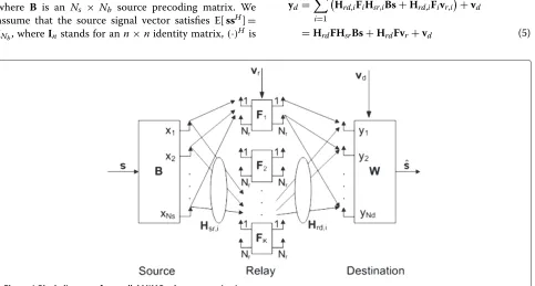
Figure 1 illustrates a two-hop MIMO relay communica-tion system consisting of one source node,Kparallel relay nodes, and one destination node. We assume that the source and the destination nodes haveNsandNd anten-nas, respectively, and each relay node has Nr antennas. The generalization to the system with different number of antennas at each relay node is straightforward. Due to its merit of simplicity, we consider the amplify-and-forward relaying scheme at each relay. The communication pro-cess between the source and destination nodes is com-pleted in two time slots. In the first time slot, theNb×1 modulated source symbol vectorsis linearly precoded as
x=B s (1)
where B is an Ns × Nb source precoding matrix. We
assume that the source signal vector satisfies E[ssH]= INb, whereInstands for ann×nidentity matrix,(·)H is
the matrix (vector) Hermitian transpose, and E[·] denotes statistical expectation. The precoded vectorxis transmit-ted toK parallel relay nodes. TheNr×1 received signal vector at theith relay node can be written as
yr,i=Hsr,ix+vr,i, i=1,. . .,K (2)
whereHsr,iis theNr×NsMIMO channel matrix between the source and theith relay nodes andvr,i is the additive Gaussian noise vector at theith relay node.
In the second time slot, the source node is silent, while each relay node transmits the linearly amplified signal vector to the destination node as
xr,i=Fiyr,i, i=1,. . .,K (3)
whereFiis theNr×Nramplifying matrix at theith relay node. The received signal vector at the destination node can be written as
yd= K
i=1
Hrd,ixr,i+vd (4)
whereHrd,iis theNd×NrMIMO channel matrix between theith relay and the destination nodes,vd is the additive Gaussian noise vector at the destination node.
Substituting (1)–(3) into (4), we have
yd= K
i=1
Hrd,iFiHsr,iBs+Hrd,iFivr,i
+vd
=HrdFHsrBs+HrdFvr+vd (5)
where we define
Hsr
HTsr,1,HTsr,2,. . .,HTsr,K
T
Hrd[Hrd,1,Hrd,2,. . .,Hrd,K]
Fbd[F1,F2,. . .,FK]
vr
vTr,1,vTr,2,. . .,vTr,KT.
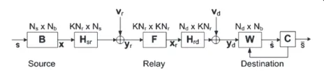
Here(·)T denotes the matrix (vector) transpose, bd[·] stands for a block-diagonal matrix,Hsris aKNr×Ns chan-nel matrix between the source node and allKrelay nodes, Hrdis anNd×KNrchannel matrix between all relay nodes and the destination node,vr is obtained by stacking the noise vectors at all relays andFis theKNr×KNr equiva-lent block diagonal relay amplifying matrix. The diagram of the equivalent MIMO relay system described by (5) is shown in Figure 2 (without the receiving filters). We assume that all noises are independent and identically dis-tributed (i.i.d.) Gaussian noise with zero mean and unit variance.
By introducing ¯
FHrdF (6)
the received signal vector at the destination can equiva-lently be written as
yd =FH¯ srBs+Fv¯ r+vd=Hs¯ +v¯
where we defineH¯ FH¯ srBas the effective MIMO chan-nel matrix of the source–relay–destination link, andv¯
¯
Fvr+vdas the equivalent noise vector. The transmission power consumed by each relay node can be expressed as
E[ tr(xr,ixHr,i)]=tr
Fi
Hsr,iBBHHHsr,i+INr
FHi
,
i=1,. . .,K
(7)
where tr(·)stands for the matrix trace. In the following, we introduce the linear MMSE receiver and the nonlinear MMSE–DFE receiver for MIMO relay systems.
Linear MMSE receiver
Using a linear receiver, the estimated signal waveform vector at the destination node in Figure 2 (without the feedback operation) is given byˆs=WHyd, whereWis an Nd×Nbweight matrix. The MSE of the signal waveform estimation is given by
Figure 2Block diagram of the equivalent MIMO relay system.
MSE=tr
Esˆ−sˆs−sH
=trWHH¯ −INb
WHH¯ −INb
H +
WHC¯vW
(8)
whereC¯vis the equivalent noise covariance matrix given by C¯v = Ev¯v¯H = F¯F¯H +INd. The weight matrixW which minimizes (8) is the Wiener filter and can be written as
W=(H¯H¯H+Cv¯)−1H¯ (9)
where(·)−1denotes the matrix inversion. Substituting (9) back into (8), it can be seen that the MSE is a function of
¯
FandBand can be written as
MSE=tr
INb+H¯
H
C−v¯1H¯ −1
. (10)
Nonlinear MMSE–DFE receiver
With a nonlinear DFE receiver employed at the destina-tion node, the source symbols are detected successively with theNbth symbol detected first and the first symbol detected last. The equivalent MIMO relay system model is shown in Figure 2. Assuming that there is no error prop-agation in the DFE receiver, the estimated source symbol vector is
¯
s=W¯Hyd−Cs=(W¯HH¯ −C)s+W¯Hv¯ (11)
whereW¯ is theNd×Nbfeed-forward weight matrix,C is theNb×Nbstrictly upper-triangle feedback matrix of the DFE receiver. To minimize the error of the signal esti-mation in (11), we haveC = U[W¯HH¯], whereU[W¯HH¯] denotes the strictly upper-triangular part ofW¯HH¯.
When the MMSE criterion is used to estimate each symbol, the feed-forward matrixW¯ is given as
[W¯]k=[H¯]1:k[H¯]H1:k+Cv¯
−1
[H¯]k, k=1,. . .,Nb
where [A]1:k stands for a matrix containing the first k columns ofA, and [A]kis thekth column ofA. Let us now introduce the following QR decomposition
G
C−
1 2
¯
v H¯ INb
=QR= ¯
Q Q
R (12)
where R is an Nb × Nb upper-triangular matrix with
all positive diagonal elements, Qis an(Nd +Nb)× Nb semi-unitary matrix withQHQ=INb,Q¯ is a matrix con-taining the firstNdrows ofQ, andQcontains the lastNb rows ofQ.
Using the QR decomposition (12), it has been shown in [13] that the feed-forward weight matrixW¯, the feedback matrixC, and the MSE matrixE=E(s¯−s)(¯s−s)Hcan be represented as
¯ W=C−
1 2
¯
v Q D¯ R−1, C=DR−1R−INb, E=D
−2
whereDRis a matrix taking the diagonal elements ofRas the main diagonal and zero elsewhere.
Minimal MMSE relay design
In this section, we address the joint source and relay optimization problem for systems with a linear MMSE receiver and a nonlinear MMSE–DFE receiver at the des-tination node, respectively. In particular, we show that for both receiver schemes, the optimal source and relay matrices have a general beamforming structure.
Optimal design with linear MMSE receiver
Based on (7) and (10), the joint source and relay optimiza-tion problem with a linear MMSE receiver used at the destination node can be formulated as
min
{Fi},B tr
INb+H¯
H
C−¯v1H¯ −1
(14)
s.t. trBBH≤Ps (15)
trFi
Hsr,iBBHHHsr,i+INr
FHi
≤Px,i, i=1,. . .,K (16)
where (15) is the transmit power constraint at the source node, while (16) is the power constraint at each relay node. Here Ps > 0 andPx,i > 0, i = 1,. . .,K, are the cor-responding power budget. Obviously, to avoid any loss of transmission power in the relay system when a linear receiver is used, there should beNb≤min(Ns,KNr,Nd).
Due to the power constraint at each relay node (16), the source and relay matrices optimization problem (14)–(16)
is much more challenging to solve when K ≥ 2
com-pared with the case ofK=1. To overcome this difficulty, we relax the power constraints in (16) by considering the power of the signal at the output of Hrd, which can be expressed as [10]
Etr(Hrdxr)(Hrdxr)H
=trF¯HsrBBHHHsr +IKNr
¯ FH
≤Pxtr(HrdHHrd).
(17)
Here, Px Ki=1Px,i is the total transmission power budget available to all K relay nodes. Using (17), the relaxed joint source and relay optimization problem can be written as
min ¯
F,B
tr
INb+H¯
H
C−v¯1H¯ −1
(18)
s.t. trBBH≤Ps (19)
trF¯HsrBBHHHsr+IKNr
¯
FH≤Pr (20)
wherePr Pxtr(HrdHHrd).
LetHsr =UssVHs denote the singular value decompo-sition (SVD) ofHsr, where the dimensions ofUs,s,Vsare
KNr×KNr,KNr×Ns,Ns×Ns, respectively. We assume that the main diagonal elements ofsare arranged in a decreasing order. The optimal structure ofF¯andBas the solution to the problem (18)–(20) is given by
¯
F=VfUHs,1, B=Vs,1b (21)
whereVis anyNd×Nbsemi-unitary matrix withVHV= INb, Us,1 and Vs,1 contain the leftmost Nb columns of Us andVs, respectively,f andbare Nb ×Nb diago-nal matrices. The proof of (21) is similar to the proof of Theorem 1 in [8]. From (21), we see that the optimal F¯ andBhave a beamforming structure. In fact, they jointly diagonalize the source–relay–destination channel H¯ up to a rotation matrixV. Using (21), the joint source–relay optimization problem (18)–(20) becomes
min
f,b
trINb+(fsb) 2(2
f +INb)
−1−1 (22)
s.t. tr2b≤Ps (23)
tr2fsb2+INb
≤Pr. (24)
Let us denote λf,i,λs,i,λb,i, i = 1,. . .,Nb, as the main diagonal elements off,s,b, respectively, and intro-duce
aiλ2s,i, xiλ2b,i, yiλ2f,i
λs,iλb,i
2+ 1,
i=1,. . .,Nb.
(25)
The optimization problem (22)–(24) can be equivalently rewritten as
min
x,y
Nb
i=1
aixi+yi+1
aixiyi+aixi+yi+1 (26)
s.t. Nb
i=1
xi≤Ps, xi≥0, i=1,. . .,Nb (27)
Nb
i=1
yi≤Pr, yi≥0, i=1,. . .,Nb (28)
where x [x1,x2,. . .,xNb]T and y [y1,y2,. . .,yNb]T. The problem (26)–(28) can be solved by an iterative method developed in [8], where in each iteration,xandy are updated alternatingly by fixing the other vector. After the optimalxandyare found,λf,iandλb,ican be obtained from (25) as
λf,i=
yi
λ2 s,ixi+1
, λb,i=√xi, i=1,. . .,Nb. (29)
Using (6) and the optimal structure ofF¯ andBin (21), we haveHrd,iFi = Vfi, where matrixi contains the
Fi=H†rd,iVfi, i=1,. . .,K (30)
where (·)† denotes matrix pseudo-inverse. Finally, we scaleFiin (30) to satisfy the power constraint (16) at each relay node as
˜
Fi=αiFi, i=1,. . .,K (31)
where the scaling factorαiis given by
αi=
Px,i
tr(Fi[Hsr,iBBHHHsr,i+INr]FHi )
, i=1,. . .,K.
(32)
Optimal design with nonlinear MMSE–DFE receiver
Using (12), (13), and the relaxed power constraint (20), the joint source and relay optimization problem which mini-mizes the MSE of the signal waveform estimation with a nonlinear MMSE–DFE receiver can be formulated as
min ¯
F,B
trDR−2 (33)
s.t. G=QR (34)
tr(BBH)≤Ps (35)
tr
¯
FHsrBBHHHsr+IKNr
¯ FH
≤Pr. (36)
Let us introduce M min(Nb, rank(Hsr)), where rank(·)denotes the rank of a matrix. The optimal source precoding matrix and the optimal relay amplifying matri-ces as the solution to the problem (33)–(36) are given by
¯
F=UfUHs,1, B=Vs,1bVHr (37)
wheref andbareM×Mdiagonal matrices,Uis any Nd×Msemi-unitary matrix withUHU=I
M,Us,1andVs,1 contain the leftmostMvectors ofUsandVs, respectively, andVr is anNb×Msemi-unitary matrix (VHr Vr = IM) such that the QR decomposition in (34) holds. The proof of (37) is similar to the proof of Theorem 2 in [13].
From (37), we find that bothF¯andBhave a beamform-ing structure. In particular, they jointly diagonalize the source–relay–destination channel matrixH¯ up to rotation matricesUandVr. It can be shown similar to [13,14] that the constraint (34) is equivalent to
d[DR]≺σG (38)
where≺stands for multiplicative majorization [15],σGis a column vector containing all singular values ofG, and d[DR] is a column vector containing all diagonal elements
ofDR. Using (37) and (38), the optimization problem (33)– (36) can equivalently be rewritten as
min
δf,δb
trDR−2 (39)
s.t. dDR2≺w
⎡ ⎣
1+
δf,iλs,iδb,i
2
δ2 f,i+1
T ,1Nb−M
⎤ ⎦
T
(40)
M
i=1
δ2
b,i≤Ps (41)
M
i=1
δ2 f,i
λs,iδb,i
2+
1≤Pr (42)
δb,i≥0, δf,i≥0, i=1,. . .,M (43)
where≺w stands for weakly multiplicative submajoriza-tion [15], 1Nb−M denotes a 1× (Nb− M) vector with all 1 elements, δf [δf,1,δf,2,. . .,δf,M], and δb [δb,1,δb,2,. . .,δb,M].
Using the definition of the operator≺win [15] and the notations of
aiλ2s,i, xi˜ δb,i2 , yi˜ δf2,i
λs,iδb,i
2+ 1,
i=1,. . .,M (44)
the optimization problem (39)–(43) can equivalently be converted to the following problem
min
˜
x,y˜
M
i=1
log aixi˜ + ˜yi+1
aixi˜yi˜ +aixi˜ + ˜yi+1 (45)
s.t. M
i=1 ˜
xi≤Ps, xi˜ ≥0, i=1,. . .,M (46)
M
i=1 ˜
yi≤Pr, yi˜ ≥0, i=1,. . .,M. (47)
Similar to the problem (26)–(28), the problem (45)–(47) can be solved by an iterative method developed in [8]. Then Fi, i = 1,. . .,K, are obtained similar to (29) and (30). Finally, the relay matrices satisfying the constraints (16) are obtained as (31) and (32).
Simulations
In this section, we study the performance of the proposed jointly optimal source and relay beamforming algorithms for parallel MIMO relay systems with linear MMSE and nonlinear MMSE–DFE receivers, respectively. All simula-tions are conducted in a flat Rayleigh fading environment where the channel matrices have zero-mean entries with variancesσs2/Ns andσr2/(KNr)forHsr andHrd, respec-tively. The BPSK constellations are used to modulate the source symbols, and all noises are i.i.d. Gaussian with zero mean and unit variance. We define SNRs = σs2PsKNr/Ns and SNRr = σr2PrNd/(KNr) as the signal-to-noise ratio (SNR) for the source–relay link and the relay–destination link, respectively. In all simulations, we set Nb = Ns =
Nr = Nd = 3 and SNRr = 20 dB. We transmit 1000Ns
randomly generated bits in each channel realization, and all simulation results are averaged over 200 channel real-izations.
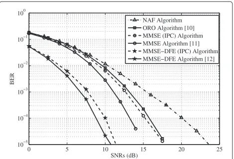
In the first example, a parallel MIMO relay system
with K=3 relay nodes is simulated. We compare the
BER performance of the following algorithms: (i) two proposed joint source and relay schemes considering individual power constraints (IPC) at each relay node; (ii) The source and relay matrices design in [11,12] with power constraint at the output of Hrd; (iii) the naive amplify-and-forward (NAF) algorithm where both the source and relay matrices are scaled identity matri-ces satisfying power constraints (19) and (20); (iv) the optimal relay only (ORO) algorithm developed in [10] where the relay matrices are optimized based on the MMSE criterion, while the source precoding matrix is a scaled identity matrix. Figure 3 shows the BER perfor-mance of six systems versus SNRs. It can be seen from Figure 3 that the NAF algorithm has the worst perfor-mance, since it does not exploit the channel knowledge available. Although both the ORO algorithm and the proposed MMSE (IPC) algorithm use a linear MMSE receiver at the destination node, the proposed algo-rithm has a better performance, since it jointly opti-mizes the source and relay matrices. We also observe from Figure 3 that as expected, the proposed optimal relay algorithm with the nonlinear MMSE–DFE receiver has the best BER performance. Note that although the algorithms in [11,12] have a better BER perfor-mance compared with the proposed algorithms, the relay matrices developed by Toding et al. [11,12] do not satisfy the power constraints at each relay node, which is more relevant for practical relay communication systems.
In the second example, we study the effect of the num-ber of relays to the system BER performance using the proposed algorithms. Figure 4 displays the system BER versus SNRs with K=2, 3, and 5. It can be seen that at BER = 10−4, for both the linear MMSE-based optimal
0 5 10 15 20 25
10−5 10−4 10−3 10−2 10−1 100
SNRs (dB)
BER
NAF Algorithm ORO Algorithm [10] MMSE (IPC) Algorithm MMSE Algorithm [11] MMSE−DFE (IPC) Algorithm MMSE−DFE Algorithm [12]
Figure 3Example 1.BER versus SNRswithK=3.
relay system and the nonlinear MMSE–DFE-based opti-mal relay system, we can achieve approximately 5-dB gain
by increasing from K=2 to K=5. We would like to
mention that although the nonlinear MMSE–DFE algo-rithm has an improved BER performance compared with the linear MMSE algorithm, the former system has a higher decoding complexity than the latter one. Such performance-complexity tradeoff is very useful for practi-cal communication systems.
Conclusions
We have derived the optimal structure of the source precoding matrix and the relay amplifying matrices for parallel MIMO relay communication systems using linear MMSE receiver and nonlinear MMSE–DFE receiver at the destination node. The proposed source and relay matrices jointly diagonalize the source–relay–destination channel and minimize the MSE of the signal waveform estimation. Simulation results demonstrate that the proposed algo-rithms have improved BER performance compared with the existing techniques.
0 5 10 15 20 25 30
10−4 10−3 10−2 10−1
SNRs (dB)
BER
MMSE (IPC) Algorithm (K=2) MMSE (IPC) Algorithm (K=3) MMSE (IPC) Algorithm (K=5) MMSE−DFE (IPC) Algorithm (K=2) MMSE−DFE (IPC) Algorithm (K=3) MMSE−DFE (IPC) Algorithm (K=5)
Competing interests
The authors declare that they have no competing interests.
Acknowledgements
This study was supported in part by the Australian Research Council’s Discovery Projects funding scheme (project number DP110100736), the Higher Education Ministry of Indonesia (DIKTI), and the Paulus Christian University of Indonesia (UKI-Paulus) of Makassar, Indonesia (PhD scholarship of Apriana Toding).
Received: 25 January 2012 Accepted: 21 July 2012 Published: 16 August 2012
References
1. B Wang, J Zhang, A Høst-Madsen, On the capacity of MIMO relay channels. IEEE Trans. Inf. Theory.51, 29–43 (2005)
2. X Tang, Y Hua, Optimal design of non-regenerative MIMO wireless relays. IEEE Trans. Wirel. Commun.6, 1398–1407 (2007)
3. O Mu ˜noz-Medina, J Vidal, A Agust´ın, Linear transceiver design in nonregenerative relays with channel state information. IEEE Trans. Signal Process.55, 2593–2604 (2007)
4. W Guan, H Luo, Joint MMSE transceiver design in non-regenerative MIMO relay systems. IEEE Commun. Lett.12, 517–519 (2008)
5. G Li, Y Wang, T Wu, J Huang, Joint linear filter design in multi-user cooperative non-regenerative MIMO relay systems. EURASIP J. Wirel. Commun. Netw.2009, Article ID 670265 (2009)
6. Y Rong, Linear non-regenerative multicarrier MIMO relay communications based on MMSE criterion. IEEE Trans. Commun.58, 1918–1923 (2010) 7. Z Fang, Y Hua, JC Koshy, Joint source and relay optimization for a
non-regenerative MIMO relay. inProc. IEEE Workshop Sensor Array Multi-Channel Signal Processing(Waltham, WA, 2006), pp. 239–243 8. Y Rong, X Tang, Y Hua, A unified framework for optimizing linear
non-regenerative multicarrier MIMO relay communication systems. IEEE Trans. Signal Process.57, 4837–4851 (2009)
9. Y Rong, Y Hua, Optimality of diagonalization of multi-hop MIMO relays. IEEE Trans. Wirel. Commun.8, 6068–6077 (2009)
10. AS Behbahani, R Merched, AM Eltawil, Optimizations of a MIMO relay network. IEEE Trans. Signal Process.56, 5062–5073 (2008)
11. A Toding, MRA Khandaker, Y Rong, Optimal joint source and relay beamforming for parallel MIMO relay networks. inProc. 6th Int. Conf. Wireless Commun., Network. Mobile Comput.(Chengdu, China, 2010), pp. 23–25
12. A Toding, MRA Khandaker, Y Rong, Joint source and relay optimization for parallel MIMO relays using MMSE-DFE receiver. inProc. 16th Asia-Pacific Conference on Communication(Auckland, New Zealand, November 1–3 2010), pp. 12–16
13. Y Rong, Optimal linear non-regenerative multi-hop MIMO relays with MMSE-DFE receiver at the destination. IEEE Trans. Wirel. Commun.9, 2268–2279 (2010)
14. Y Jiang, W Hager, J Li, The generalized triangular decomposition. Math. Comput.77, 1037–1056 (2008)
15. AW Marshall, I Olkin,Inequalities: Theory of Majorization and Its Applications (Academic Press, New York, 1979)
doi:10.1186/1687-6180-2012-174
Cite this article as:Todinget al.:Joint source and relay optimization for par-allel MIMO relay networks.EURASIP Journal on Advances in Signal Processing
20122012:174.
Submit your manuscript to a
journal and benefi t from:
7Convenient online submission
7Rigorous peer review
7Immediate publication on acceptance
7Open access: articles freely available online 7High visibility within the fi eld
7Retaining the copyright to your article