Using Linear Parameter-Varying Models
Pawel Majecki*, Gerrit M. van der Molen*, Michael J. Grimble*, Ibrahim Haskara**, Yiran Hu**, Chen-Fang Chang**
*Industrial Systems and Control, Glasgow, UK (e-mail: [email protected])
**General Motors R&D, Propulsion Systems Research Lab, Warren, MI 48090 (e-mail: [email protected])
Abstract: As a response to the ever more stringent emission standards, automotive engines have become more complex with more actuators. The traditional approach of using many single-input single output controllers has become more difficult to design, due to complex system interactions and constraints. Model predictive control offers an attractive solution to this problem because of its ability to handle multi-input multi-output systems with constraints on inputs and outputs. The application of model based predictive control to automotive engines is explored below and a multivariable engine torque and air-fuel ratio controller is described using a quasi-LPV model predictive control methodology. Compared with the traditional approach of using SISO controllers to control air fuel ratio and torque separately, an advantage is that the interactions between the air and fuel paths are handled explicitly. Furthermore, the quasi-LPV model-based approach is capable of capturing the model nonlinearities within a tractable linear structure, and it has the potential of handling hard actuator constraints. The control design approach was applied to a 2010 Chevy Equinox with a 2.4L gasoline engine and simulation results are presented. Since computational complexity has been the main limiting factor for fast real time applications of MPC, we present various simplifications to reduce computational requirements. A benchmark comparison of estimated computational speed is included.
Keywords: SI engines, model predictive control, nonlinear control, LPV models
I. INTRODUCTION
In order to meet more stringent future emissions standards as well as the desire for better engine performance, engine control systems have become more complex. Dual independent cam phasing, that was rare, is now widely used. Each actuator needs to be controlled to a setpoint, such that the overall engine performance, which is assessed based on the opposing objectives of drivability, emissions and fuel economy, is optimized. Coordination of the various engine actuators has always been difficult. Traditionally, each actuator was controlled to its own setpoint based on engine operating condition. A large effort is required to calibrate the set-points offline so that the real-time control of the actuators does not result in undesirable behaviour. Moreover, ad-hoc patches are also often needed so that good performance is achieved under transient conditions. To avoid having too many patches, setpoints are selected to be conservative,
which makes the engine controls difficult to calibrate.
The difficulty with the engine control problem is that the system is nonlinear, multi-input multi-output (MIMO), and has many actuator and state/output constraints. The shortcomings of the traditional single-input single-output (SISO) design philosophy are therefore becoming more evident. Model based control design can potentially provide a solution, which is truly multivariable, more flexible, and easier to upgrade when engine configurations change. Of the
many advanced control design methodologies available, model predictive control (MPC) is a popular control strategy because of its ability to tackle multivariable processes, handle constraints, deal with long time-delays, and utilize future reference knowledge. The main disadvantage of MPC controllers is that they can be computationally intensive due to the online optimization process used to compute the current control. Quadratic programming (QP) usually provides the most efficient optimization algorithm, but this in principle only applies to linear models. Early work on MPC focused on linear time-invariant (LTI) systems. Popular predictive algorithms are Dynamic Matrix Control (Cutler and Raemaker, 1979), Generalized Predictive Control (GPC), due to Clarke et al. (1989), and those due to Richalet (1978). For useful review papers on MPC see Bemporad and Morari (2004), Qin and Badgwell (2003), and the references therein.
behaviour and require sampling times of a few milliseconds. This poses a challenging problem requiring tailored NL predictive control methods. With advances in computing power, it has been possible to apply MPC in high bandwidth control applications, including automotive systems. Nonlinear MPC for automotive engines was considered by Herceg et. al. (2006) and Vermillion et. al. (2010).
Another area of active research is control design based on Linear Parameter Varying (LPV) models. This class of models provides can approximate nonlinear systems whose nonlinearity enters via parametric changes. The application of LPV models to MPC provides a great middle ground between traditional LTI model-based MPC and the less-attainable full nonlinear MPC. The QP optimization methods can be used, because LPV models are quasi-linear, providing an efficient solution method. Due to this improved modelling approach, MPC may now be used on some applications, where it was previously unsuitable (see for example Casavola et al 2002, 2003; Chisci 2003; Besselmann 2012; Li 2010, Duan 2013). The main contribution in the following lies in the formulation of the Nonlinear Generalized Predictive Control (NGPC) problem in a useful form for the engine control application.
In the following, an engine control that uses an LPV model-based MPC solution is proposed. The problem of MIMO torque and air-fuel-ratio (AFR) control is considered. These are two of the most critical variables in the engine control system, which have a direct influence on drivability, emissions and fuel economy. The desired engine torque depends upon the driver’s pedal position. The intake throttle is the main actuator to control the intake manifold pressure and thus the inducted air charge. This in turn controls the engine torque. In addition to torque delivery, engine control systems also need to address other objectives such as improved fuel economy, reduced engine-out and tailpipe emissions. For a SI engine, AFR must be regulated, to achieve good emissions through torque transients.
II. ENGINE CONTROL PROBLEM
The problem of engine torque and air-to-fuel ratio control is considered in this paper. The engine is the 2.4L engine used on a 2010 Chevy Equinox. Amongst the main characteristics of this particular engine are dual independent cam phasers and a direct fuel injection system. The general block diagram of the engine torque and AFR production process is shown in Fig. 1. The throttle is used to maintain intake manifold air pressure. As cylinders go through an induction cycle, air is drawn into the cylinders through the intake valves. Cam phasing changes the intake/exhaust valve opening and closing timing, which varies the amount of trapped residual and the fresh charge in the cylinder. The FPW command, applied to the injectors determines the amount of fuel injected into the cylinders. The injected fuel is mixed with the air charge and is then ignited during the compression cycle. Spark timing controls the ignition time, and this determines the combustion phasing and the final torque generated during that combustion event.
The desired engine torque is determined by the accelerator pedal position interpreting the driver request. The desired
AFR is a function of the type of fuel used, as well as operating conditions. For stoichiometric SI engine, the desired AFR is the stoichiometric AFR for the recommended fuel. In some cases, a richer or leaner AFR may be required for other reasons (such as piston protection). Note that there are non-stoichiometric operating SI engines, where the desired AFR will vary significantly depending on the load.
Fig. 1: Block diagram of the SI Engine
There are primarily five actuators that control the engine torque and AFR, namely throttle position, fuel pulse width (FPW), intake and exhaust cam phaser angles, and the spark advance. With the direct fuel injection system, there is a simple relationship between the FPW and the cylinder fuel charge. The throttle position and CFC are the two manipulated inputs, resulting in a square system. The ICAM and ECAM phaser position set-points, and the spark advance are obtained from operating-point dependent tables optimized to produce the best torque (MBT), and a desired trade-off between fuel economy and drivability. In this work these are treated as known disturbance inputs. The set of measurements available include Manifold Absolute Pressure (MAP) in the intake manifold, Mass Air Flow (MAF), air charge temperature (MAT), throttle position (TPS), exhaust AFR, cam phaser positions, engine speed, ambient pressure and ambient temperature. The sensors can be used for feedback control and to update model parameters.
III. ENGINE LPV MODEL
the physics-based filling and emptying model. Regression models are available for static components, such as volumetric efficiency and engine torque output. A first-order order lag was used to model the lambda sensor. Transforming a physics based model into an LPV form is therefore more advantageous than the data identification approach.
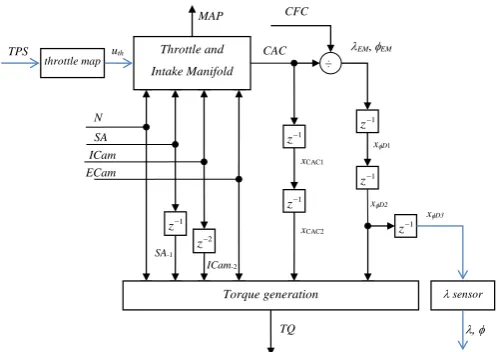
During the model development, throttle and fuel injector dynamics were ignored, a one-state intake manifold model was used and engine rotational dynamics were not included (engine speed was considered an external parameter). Model parameters were estimated using driving cycle data, and the model was transformed to a quasi-LPV form by exploiting the natural physical structure of the solution. The engine hybrid model is an interconnection of the continuous-time intake manifold and lambda sensor dynamics, and the event-based mean-value models for the volumetric efficiency, torque production and exhaust manifold dynamics. The model for the control design was defined in an event-based time-frame, and consists of the Euler-discretized intake manifold, and lambda sensor dynamics in combination with explicit discrete-time delays. Fig. 2 shows the block diagram of the engine used for control design.
TQ N
SA ICam ECam
÷
λ sensor
1
z−
2
z−
1
z− CFC
CAC λEM, φEM
λ, φ Torque generation
Throttle and Intake Manifold TPS
SA-1
ICam-2 1
z−
1
z−
1
z−
1
z− xCAC1
xCAC2
xφD1
xφD2
xφD3
MAP
[image:3.595.42.291.340.516.2]throttle map uth
Fig. 2: Structure of Engine Model for Control Design (delay blocks represent discrete engine event time steps)
The model has 7 states: intake manifold pressure Pim, two delayed CAC states xCAC1-2, three delayed in-cylinder equivalence ratio states xφD1-3 and the state φ representing the output of lambda sensor. The outputs are the generated torque TQ and the in-cylinder fuel-air ratio φIC. The manipulated control variables are the Throttle Position (TPS) and Cylinder Fuel Charge (CFC). The LPV model used in the MPC
controller suggested use of the quadratic function of the throttle area Ath as the effective control variable uth:
1 ( 1)
th th CdA CdAx th
u = A ⋅p ⋅ p A + (1)
The parameter pCdAx is defined such that the function has a maximum at Ath,max, i.e. for TPS = 100%. The throttle position TPS can be retrieved from uth using a one-to-one mapping. The equivalence ratio φIC, rather than the air-fuel ratio λIC, was chosen as the output to be controlled,
exploiting its proportionality to the control input CFC. The state, input, and the controlled and measured output vectors:
0 1 2 3 1 2
T
im D D D CAC CAC
x = P φ xφ xφ xφ x x
, ,
th
c m
IC
MAP TQ
u
u y y TQ
CFC φ
φ
= = =
(2)
State Equation Matrices: The discrete-time LPV model of the engine with both measured (ym) and controlled (yc) outputs is written in general form as:
0, 1 0 0, 0 ,
, 0 0, ,
, 0, ,
t t t t t k x t
m t mt t mt t k ym t
c t ct t ct t k yc t
x A x B u d
y C x E u d
y C x E u d
+ −
− −
= + +
= + +
= + +
(3)
where k is the common input delay and the notation Xt denotes X(pt), i.e. an LPV matrix evaluated based on the values of parameters at time t. The terms dx, dym and dyc represent known input signals other than the control u. The parameter vector in this problem contains the following variables p = (N, MAP, SA, ICAM, ECAM, Tim, Pamb, Tamb). Apart from the exogenous signals it also contains a system state (MAP), making the model quasi-LPV. The state matrices
A0(pt) and B0(pt) can be constructed as:
0 0
1 0 0 0 0 0 0
0
0 0
0 1 0 0 0 0
0
0 0 0 0 0 0 0
,
0 0
0 0 1 0 0 0 0
0 0
0 0 0 1 0 0 0
0 0
0 0 0 0 0 0
0 0
0 0 0 0 0 1 0
cyl im
s s
cyl air im
V V
t t
Stoich CAC
A B
V R T
λ λ
η
τ τ
η
−
Ω
−
= =
where Ω =ts Rair im ambT P ⋅ Ψ ⋅ +
(
1 pCdA2Pim)
TambVim.These matrices, that are measured, or estimated, at time t,
contain both constant and varying engine parameters. The volumetric efficiency η(⋅), throttle function Ψ(Pim/Pamb) and the cylinder air charge CAC expressions are given as:
3 3 2
1 2 3
2 2
4 5 6 7 8 9
2 2
10 11 12 13
( im, , , ) VE VE im VE
VE im VE VE im VE VE VE
VE VE VE im VE im
P N ICam ECam p N p P p N
p P p N p P p p ICam p ICam
p ECam p ECam p N P p NP
η = + + +
+ + + + +
+ + + +
(4)
1 1
1
1
2( 1) 1
2 2
1 ,
1 1
( )
2 2
1 1
pr pr pr
pr
pr
γ γ
γ
γ γ
γ γ
γ γ
γ
γ γ
γ
γ γ
−
−
+
− −
− >
− +
Ψ =
≤
+ +
( )
ac s cyl air im im
CAC=m ⋅ =t V R T ⋅ ⋅η P (6)
0.5[ ] 60[ / min] [ / min]
s
t = rev ⋅ s N rev (7)
The effective disturbance input dx,t is zero in this LPV model. Indeed, all the disturbance inputs form elements of the LPV
state matrices. From the definition of the measured and controlled outputs in (2), the output LPV matrices are:
0 3 2 0 ,
1 0 0 0 0 0 0 0
0 0 0 0 0 , 0,
0 1 0 0 0 0 0 0
m TQ TQ m ym TQ t
C p p E d d
= = =
3 2
, ,
,
0 0 0 0 0
0 0 0 0 0 0 0
0 0
0 0
TQ TQ
t
c t t
EM t
TQ t t t
p p
TQ
y x
d u Stoich
CAC φ
= =
+ +
The output torque components due to disturbance inputs:
2 2
1 4 1 5 1 6 7 8 1
2 2 2
9 1 10 2 11 2 12 13
TQ TQ TQ TQ TQ TQ TQ
TQ TQ TQ TQ TQ
d p p SA p SA p N p N p SA N
p SA N p ICam p ICam p ECam p ECam
− − −
− − −
= + + + + + ⋅
+ ⋅ + + + +
The volumetric efficiency and cam angles appear as LPV parameters; RPM appears indirectly through sample time; dependence of the discharge coefficient on the MAP state is taken into account by a term in the B0 matrix (demonstrates
quasi-LPV nature of the model). The control inputs uth and
CFC appear linearly in the equations, with the control signal
uth depending uniquely on the throttle position TPS and not on the state MAP. The terms in the torque model that are not model states appear as measured disturbance terms.
The above LPV model formulation is not unique. In fact, pointwise controllability and achievable performance depend on the choice of the model, even though the open-loop characteristics remain unaffected (Huang and Jadbabaie, 1999). This is a feature of quasi-LPV models. In some cases the model formulation follows naturally from the system structure, but in general the "best" formulation may not be obvious. The model does not rely on Jacobian linearization, i.e. it is valid for the whole range of engine operating conditions, limited only by the validity of the NL model.
IV. CONTROLLER DESIGN
There are many possible formulations and variations of the predictive control problem. The Nonlinear Generalized Predictive Controller (NGPC) algorithm used here seems well suited to real-time engine control applications. At each time step, the controller aims to minimize the sum of squares of predicted performance variables, with or without constraints on the control signal changes. The traditional method of introducing integral action in predictive control is to augment the system input by adding an integrator:
, 1 ,
,
i t i t t k
t k i t t k
x x u
u x u
β β
+ −
− −
= + ∆
= + ∆
(8)
1
(1 (1 ))
t k t k
u− = −βz− ∆u− (9)
The MPC cost function normally contains a penalty on the incremental change in control action ∆ut . The error weighting matrices can in this case just be constant matrices (no extra states). It is useful to define a generalized operator
in unit-delay terms ∆ = −β (1 βz−1) so that if β = 0 then ∆βut k− =ut k− . The results therefore apply to both
systems using control input and rate of change of control input, respectively. If β =1 equation (9) defines an integrator without additional delay. If the actual control input ut is used, an alternative way of including integral action is to use a dynamically weighted error signal involving a high gain in low frequencies. The steady-state error should then be removed, otherwise the cost would increase indefinitely.
Performance variables and combined model: The output
variables of interest are contained in the vector yc:
, ,
c t ct t ct t k yc t t
y =C x +E ∆βu− +d +c (10)
The controlled output yc can be different from the measured output ym. A ‘robustness’ signal ct is included in an output disturbance model, to compensate for modelling mismatch:
, 1 ,
,
d t d d t d t
t dc d t
x
A x
B
c
C x
ω
+
=
+
=
(11)It is often desirable to consider dynamically weighted performance variables, to penalize the signals in different frequency ranges. In fact, it may also be useful to penalize actuator movements to prevent too aggressive (high-frequency) control actions. This motivates an introduction of dynamic weighting functions acting on the control error
,
(rt−yc t) and possibly on the control action ut:
1
, ( )( , )
p t e t c t
e =W z− r −y : , 1 , ,
, , ,
( )
( )
p t p p t p t c t
p t p p t p t c t
x A x B r y
e C x E r y
+ = + −
= + −
(12)
The augmented statext = x0Tt,xdtT,xitT,xTptTfor the combined
model and vector of performance variables, including weighted error z=epfollows:
0, 1 0 0 0
, 1
, 1
, 1
0 0 0
0 0
0 0 0
0 0 0
0 0
0 0 0 0
0 0 0 0
0 0
t t
d t d dt
i t it
p c p dc p c p pt
p t
t d
t k
t
p c p p c
x A B x
x A x
x I x
B C B C B E A x
x
B G D
r B
u
I d
B E B B H
β
β
β β
+
+
+
+
−
=
− − −
+ ∆ + +
− −
t t
ξ ω
t
p c t k p p c
t
r
E E u E E H
d
β −
+ − ∆ + −
More concisely: 1 ,
,
t t t t t k x t t
t t t t t k y t
x A x B u g D
z C x E u g
β
β
ζ
+ −
−
= + ∆ + +
= + ∆ +
(13)
The model (13) defines the variables to be minimized. The dynamic control weighting is not used here, i.e. Wu = I. Limiting the controller bandwidth can also be achieved by using the constrained solution. The control law derivation summarized below is in Grimble and Majecki (2010).
Cost Function and Prediction Equations: At each sample instant, the predictive controller minimizes a criterion over a cost horizon N, involving a weighted combination of the predictions of performance variables and the control effort:
(
)
(
)
1
0 ( )
N T
T
t t k i t k i t i u t i
i
J N z z βu βu
−
+ + + + + +
=
= + ∆ Λ ∆
∑
(14)Note the time shift of k sample time steps between the two quadratic terms in the cost, reflecting the fact that the control at the current time t can only affect the output with a k-steps delay. For simplicity, it will be assumed that k = 1. Consequently, the solution involves the initial step of computing the k-step state prediction. The cost (14) can then be represented in a vector-matrix form as:
(
)
(
)
, , , ,
T T
N t k N t k N t N U t N
J =Z+ Z+ + ∆βU Λ ∆βU (15)
where , 1 , 1
1 1
,
t t k
t t k
t k N t N
t N t k N
u z
u z
Z U
u z
β β β
β
+
+ + +
+
+ − + + −
∆
∆
= ∆ =
∆
(16)
The future values of the performance variables z are estimates given the information available at time t. They are based on the state estimates (provided by the Kalman Filter), current measured disturbances (assumed to stay constant within the prediction horizon), the reference signal (with or without future knowledge), previous control actions and the control input sequence ∆βUt−1,N (computed in the previous iteration). The aim is to find the control sequence ∆βUt N,
that minimizes the cost (15). Invoking the receding horizon strategy, only the first element of the sequence is applied.
To minimize the cost index equations are needed to predict future values of performance variables. Based on (13), setting the stochastic noise inputs to zero, the state predictions:
1 2 1 2 1
1 2 2 1 1 1 2 2
1 1 1 2 1 ,
1 2 2 , 1 , ,
t j t j t j t t t j t j t t t
t j t j t t t t j t j t j
t j t j t j t j t x t
t j t j t x t t j x t x t
x A A A x A A A B u
A A A B u A B u
B u A A A g
A A A g A g g
β
β β
β
+ + − + − + − + − +
+ − + − + + + + − + − + −
+ − + − + − + − +
+ − + − + + −
= + ∆
+ ∆ + ∆
+ ∆ +
+ + +
or xt+j =xt0+j+xtd+j+st jx, ∆βUt N, (17)
Note that xt0+j = At+ −j 1At+ −j 2A xt t represents the free
response, xtd+j the forced response and ∆βUt N, the optimization variables. The j-step-ahead prediction follows:
(
)
, 0
, , ,
t j t j t j t j t j k y t
x d
t j t j t N t j t j k t j t j t j y t
z C x E u g
C s U E u C x x g
β
β β
+ + + + + −
+ + + − + + +
= + ∆ +
= ∆ + ∆ + + +
, ,
t j t N t j
s βU f+
= ∆ + (18)
where st j, =Ct+j t jsx, +Et+j (19)
(
0)
,
d
t j t j t j t j y t
f+ =C+ x+ +x+ +g (20)
Finally, the vector Zt+k,N can be written as:
, , , ,
t k N t N t N t N
Z+ =S ∆βU +F (21)
, ,1 ,2 , , 1 2
withSt N =stT sTt st NT T,Ft N =ftT+ ftT+ ft NT+ T
Due to the k-steps delay, the prediction equations (17) are shifted by (k-1) steps. The starting point for predictions is not the current xˆt but xˆt k+ −1. This can be computed from the
previous controls assuming no future disturbance changes.
The parameter-dependent matrices in the above expressions are computed based on the future predicted states in (17). Alternatively, they can be found, at each control calculation, using the current state estimate xt(frozen model). This results in a less computationally demanding algorithm but there is a loss of model accuracy. The future control sequence is needed to compute the future state estimates. An iterative "successive approximation" procedure can be used to improve predictions but adding to the computational burden.
Unconstrained and Constrained Solutions: The
unconstrained minimum of the cost-function (15), given the prediction equation (21), is computed from a simple gradient calculation, or by completing the squares, to obtain:
(
)
1, , , , ,
T T
t N t N t N U t N t N
U S S S F
β
−
∆ = − + Λ (22)
min t N, max
Y ≤Y ≤Y . They can be written in the linear matrix
inequality form: M∆βU∆βUt N, ≤b∆βU (23)
The control magnitude and rate are related as:
1 2
1 1
0 0
0 0
0 0
t t t t t
C C
I I
I I
U U U u U
I I
− −
−
−
∆ = − = +
−
(24)
3 4
1
0 0
0
t t t
C C
I I
I I I
U u U
I I I I
−
= + ∆
(25)
The output constraints can be represented in the standard form by writing the outputs in a form similar to (21):
1, , , ,
Y Y
t N t N t N t N
Y+ =S U +F (26)
with appropriate definition of St NY, andFt NY, . The minimum of (15), subject to the constraints, can be obtained by quadratic programming, using the Hildreth algorithm (Wang, 2009).
Time-Varying Kalman Filter: To construct the prediction matrices St N, andFt N, the NGPC controller relies on the system states to be available at the current time t. These may be measured but a Kalman filter is used in practice to estimate them. The filter makes uses of the LPV model of the engine, the measurable disturbances and outputs. The process model and sensor noise covariances can be used as filter tuning parameters. The filter provides the state estimates including disturbance and the dynamic weighting states. The system model (13) includes stochastic white noise sources
T
T T
t t t
ς = ξ ω
and vt, representing process and measurement noise and can be written as:
1 ,
,
t t t t t k x t t
mt mt t mt t k ym t t
x A x B u g D
y C x E u d v
β
β
ζ
+ −
−
= + ∆ + +
= + ∆ + +
(27)
The covariance matrices of the signals ςt and vt are denoted
QN and RN, respectively. These can be treated as tuning parameters, used to define the relative ‘confidence’ in the model and the measurements. The D matrix is used when there is more detailed knowledge about the system stochastic properties. When there is little information the D can be set to identity and then process noise directly represents the uncertainty associated with the estimation of the particular state. The part of the D matrix associated with the white noise input ωt corresponds to the output disturbance model, including mismatch states. The signal ut-k is fed to the
Kalman Filter, as in Fig. 3. At time t, the time-varying Kalman Filter equations involve two steps:
Step 1: Computation of the Kalman gain, state estimation and update of the estimation error covariance (system matrices evaluated with the state prediction xˆt t| 1− ):
(
)
1| 1 | 1 | 1 | 1 | 1 | 1
T T
t t t t t t t t t t t t N
K − =P −C − C −P −C − +R − (28)
(
)
| | 1 | 1 , | 1 | 1 , ,
ˆt t ˆt t t t m t t t ˆt t m t t k ym t
x =x − +K − y −C −x − −E u− −d (29)
| | 1 | 1 | 1 | 1
t t t t t t t t t t
P =P − −K −C −P − (30)
Step 2: State and covariance matrix predictions (system matrices evaluated with the state estimatexˆt t| ):
1| | ,
ˆt t t t tˆ t t k x t
x+ =A x +B u− +g (31)
1| |
T T
t t t t t t N
P+ =A P A +DQ D (32)
The model mismatch may result in a steady-state offset in the system output estimate which can sometimes be compensated by representing the mismatch by an output disturbance.
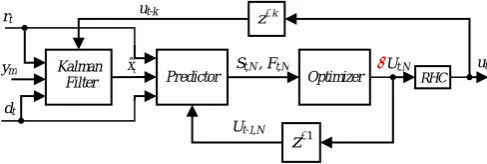
MPC Controller Structure: The overall NMPC controller structure in Fig. 3 is a form of separation principle and consists of the Kalman filter, state predictor and optimizer. The RHC block represents the receding horizon control strategy, whereby only the first element of the computed control sequence is used for actual control. The remaining elements are utilized for future state predictions.
MPC Design Issues and Weightings: The cost-function
[image:6.595.306.550.592.674.2]utilized is general using dynamic cost-function weightings. The sample time and prediction horizon N should be set so that the dominant transient behaviour is captured. There is a choice between the absolute and incremental control formulations. The ‘∆u’ approach is the classical approach. Integral action can also be added (when penalizing the control u) by including an integrator on the error weighting. The dynamic error and control weightings We(z-1) and Wu(z-1) are usually chosen to have low pass and high pass characteristics, respectively, and a constant control weighting matrix Λu may be used. The actuator and operating constraints (for QP computations) and the QN and RN covariance’s for the Kalman Filter are also design variables.
Fig. 3: MPC Block Diagram Including Kalman Filter
V. NGPC CONTROL SIMPLIFICATIONS
The predictive control algorithm as detailed in the previous section may result in an excessive computational burden on the production control processing unit, particularly when both
rt
ym
dt
ˆt
x Kalman
Filter Predictor Optimizer
k
z−
1
z−
RHC St,N , Ft,N ∆Ut,N ut
the sampling frequency and prediction horizon are high, and the constrained solution is used. For practical implementation the controller code must execute in real time in a deterministic way. The additional caveat in engine control is that the sample period varies with engine cycle and is dependent on the engine speed. Since all the code is executed at each trigger, it must have sufficient time to complete for the highest expected engine speed. Alternatively, the number of flops required may need to be reduced. The simplest way to reduce the numerical load is to reduce the horizon N. From (22), the MPC solution involves inverting at each step a matrix of size N, which has complexity O(n3). Even a small reduction of N can then bring significant computational savings, resulting in some degradation of performance. It is therefore important to strike the right balance between the algorithm complexity and the performance demanded.
Freezing Prediction Model: The state and output predictions performed at each step in (17) and (18) involve LPV model matrices, which in general vary with external parameters and/or system states. Consequently, these matrices need to be evaluated N times at each step. A simple way to reduce the number of computations is to fix the prediction model based on the parameters and states available at the current time t
and use them for prediction as in the linear GPC case.
Connection Matrix and Control Profile: At each step, the
MPC optimization problem with prediction horizon N
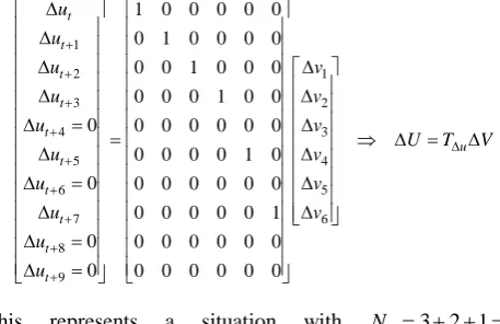
involves the computation of N decision variables (control moves). With a large N, this may lead to over-parameterization and an impractical solution. One commonly used solution is to introduce a separate control horizon Nu which uses the first Nu controls as the decision variables, and fixes the remaining (N–Nu) ones. Here we generalize this idea by defining a control profile Pu of the form:
row{Pu} = [number of samples held, repetitions] (33)
For example, letting Pu = [1 3; 2 2; 3 1] represents 3 different initial controls, then 2 samples with the same control used but this is repeated again, and finally 3 samples with the same control used. Based on a control profile, it is possible to specify the transformation matrix Tu, relating the control moves to be optimized (say vector V) to the full control vector (U). For incremental control, the connection matrix:
1
2 1
3 2
4 3
5 4
6 5
7 6
8
9
1 0 0 0 0 0
0 1 0 0 0 0
0 0 1 0 0 0
0 0 0 1 0 0
0 0 0 0 0 0 0
0 0 0 0 1 0
0 0 0 0 0 0 0
0 0 0 0 0 1
0 0 0 0 0 0 0
0 0 0 0 0 0 0
t t t t t
t t
t t t
u u
u v
u v
u v
u v
u v
u v
u u
+
+
+
+
+
+
+
+
+
∆
∆
∆ ∆
∆ ∆
∆ = ∆
=
∆ ∆
∆ = ∆
∆ ∆
∆ =
∆ =
u U T∆ V
⇒ ∆ = ∆
This represents a situation with Nu = + + =3 2 1 6 independent control moves and N= × + × + × =3 1 2 2 1 3 10 sample points. The computation of 4 control moves has been
avoided, representing a substantial computational saving. This approach, often termed ‘move blocking’ in the MPC literature, can provide the solution to the GPC class of problems with different control and error horizons. The changes to the algorithm are minimal. It also solves the problem where the horizons are the same but the control changes are not allowed at each sample instant. The usual approach is to assume future control changes are null after the control horizon Nu and in this case the connection matrix can be defined to have Nu+1 rows and N+1 columns. For example, the form of the Tumatrix, when N = 6 and Nu = 2:
, , 1 2
1 0 0 0 0 0 0
0 1 0 0 0 0 0
0 0 1 0 0 0 0
and 0 0 0 0
T
u
T
T T T
t N u t Nu t t t
T
U T U u u+ u+
=
∆ = ∆ = ∆ ∆ ∆
VI. RESULTS
Two simulation scenarios are presented here. Fig. 4 shows the comparison between the nominal MPC design and the conventional controller for a fragment of an FTP drive cycle. Extended prediction horizon and handling system interactions by the multivariable controller generally lead to improved tracking for both torque and lambda output signals. The more aggressive MPC causes overshoots at low/negative torques, however in reality this operating range would be handled by a separate idle speed controller.
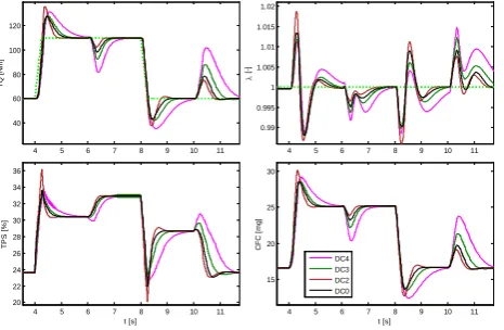
The responses to torque reference and speed disturbance step changes for different MPC designs are shown in Fig. 5. The nominal case DC0 was based on the absolute control formulation (β = 0), constrained solution and equal horizons
[image:7.595.50.279.586.734.2]N = Nu = 15. The other design cases represent various design simplifications and are listed in Table 1, where their relative speed-up factors are also benchmarked against the nominal. Analysis of the figures and table leads to several conclusions. First, freezing the prediction model (neglecting the time variation of state matrices) gives almost 20% speed-up without changing the results noticeably (this case was not included in the figure). As expected, reducing the prediction horizon significantly reduces the computational load, however the dynamic performance also changes substantially. On the other hand, the use of separate control horizon or control profile/connection matrix allows reducing the load without degrading performance.
Table 1 MPC Design Cases and speed-up factors due to the algorithmic simplifications used
DC Configuration Speed-Up (%)
0 Nominal design case (N = 15) 0.0
1 Prediction model frozen 19.3
2 Unconstrained solution 48.5
3 N = 12 3.1
4 N = 9 18.4
5 N = 6 39.7
190 192 194 196 198 200 202 204 206 208 210 0.98
0.985 0.99 0.995 1 1.005 1.01 1.015 1.02 1.025
λ
[-]
190 192 194 196 198 200 202 204 206 208 210 -40
-20 0 20 40 60 80 100 120 140
T
Q [N
m
]
190 192 194 196 198 200 202 204 206 208 210 0
5 10 15 20 25 30 35 40 45
T
P
S
[
%
]
t [s] 190 192 194 196 198 200 202 204 206 208 210
0 5 10 15 20 25 30
CF
C [
m
g
]
t [s]
[image:8.595.44.290.71.232.2]Baseline NGPC TQSP
Fig. 4: Comparison of the classical (red) and MPC (black) control for a fragment of FTP cycle
4 5 6 7 8 9 10 11
0.99 0.995 1 1.005 1.01 1.015 1.02
λ
[
-]
4 5 6 7 8 9 10 11
40 60 80 100 120
T
Q
[
Nm
]
4 5 6 7 8 9 10 11
20 22 24 26 28 30 32 34 36
T
PS [
%
]
t [s]
4 5 6 7 8 9 10 11
15 20 25 30
CF
C [
m
g
]
t [s] DC4 DC3 DC2 DC0
Fig. 5: Responses to torque reference and speed disturbance step changes for MPC design (cases: DC0 (black), DC2 (red), DC3 (green) and DC4 (magenta))
In fact, down-sampling the control action may lead to performance improvement. The unconstrained solution is also less computationally expensive and is always considered an option. For the constrained version, computational savings can also be obtained by reducing the number of the active-set iterations in the QP algorithm. As this is related to convergence of the algorithm, this step must be taken carefully by gradually reducing the number of iterations.
VII. CONCLUSIONS
The LPV-based version of the predictive control law is computationally intensive, although simpler than most nonlinear predictive algorithms. Attention therefore turned to simplifications to the controller, to reduce the computational load. We considered the application to the engine control problem and benchmarked the performance. The impact of code optimization was assessed, and the results show significant savings are possible through a combination of measures to modify the standard design process and simplify the algorithm. These were validated during the trials of embedded engine control code.
The value of this work also lies in the systematic framework for NL MPC based on quasi-LPV models, including absolute and incremental control. The use of an output disturbance model to reduce the effects of plant-model mismatch is useful, as is the way of limiting the control moves to gain computational savings. The simulation results for the torque tracking and air-fuel ratio regulation problem were shown. On-going work involves the use of variable cam phasing to improve fuel economy and real-time implementation.
REFERENCES
Bemporad, A and M Morari, (2004), Robust model predictive control: A survey, in Proc. European Control Conference, Porto.
Clarke, D.W., and C. Montadi, (1989), Properties of generalised predictive control, Automatica, Vol. 25, No. 6, pp. 859-875.
Cutler C.R. and Ramaker B.L. (1979), Dynamic matrix control - A computer control algorithm, A.I.C.H.E, 86th National Meeting
Grimble M.J. and P. Majecki (2010), State-space approach to nonlinear predictive generalized minimum variance control, International Journal of Control, Vol. 83, pp.1529-1547.
Herceg M., T. Raff, R. Findeisen and F. Allgöwer, (2006), "Nonlinear model predictive control of a turbocharged engine", Proc. 2006 IEEE Int. Conf. on Control Algs, Munich, pp. 2766-71
Huang Y. and A. Jadbabaie, (1999) Nonlinear H-infinity control: an enhanced quasi-LPV approach, IFAC World congress, Beijing.
Jankovic M., (2002) "Nonlinear control in automotive engine applications", Proceedings of 15th MTNS Conf., South Bend, IN.
Qin, S and T Badgwell, (2003), A survey of industrial model predictive control technology, Con. Eng. Prac., Vol. 11, pp. 733-764
Richalet J., A. Rault, J.L. Testud, J. Papon (1978), Model predictive heuristic control applications to industrial processes, Automatica, 14, pp. 413-428.
Vermillion C, K Butts, and K Reidy, (2010), Model Predictive Engine Torque Control, ACC, Baltimore.
Wang L., (2009) Model Predictive Control System Design and Implementation Using Matlab, Springer.
Casavola, A, Famularo, D and G Franzè, 2003, Predictive control of constrained nonlinear systems via LPV linear embeddings, Int. Jour of Robust and Nonlinear Control, Vol.13; Issue 3-4; pp. 281–294.
Chisci, L., F, Paola and G Zappa, 2003, Gain-scheduling MPC of nonlinear systems, Int Jour. of Robust and Nonlin Cont., 13; pp.3-4.
Casavola, A., Famularo, D. and G Franze, 2002, A feedback min-max MPC algorithm for LPV systems subject to bounded rates of change of parameters, IEEE Trans. A.C, ,47, No.7, pp.1147-1153.
Besselmann, T., J. Lofberg. and M Morari, 2012, Explicit MPC for LPV Systems: Stability and Optimality, IEEE Transactions on Automatic Control, vol.57, No.9, pp.2322-2332.
Li D., and Y. Xi, 2010, The Feedback Robust MPC for LPV Systems With Bounded Rates of Parameter Changes, IEEE Trans. on Automatic Control, vol.55, No.2, pp.503-507, Feb., pp.503-507.
[image:8.595.47.280.289.441.2]