Ramanujan graphs in cryptography
Anamaria Costache1, Brooke Feigon2, Kristin Lauter3, Maike Massierer4, and Anna Pusk´as5
1
Department of Computer Science, University of Bristol, Bristol, UK, [email protected] 2Department of Mathematics, The City College of New York, CUNY, NAC 8/133, New York, NY 10031,
3Microsoft Research, One Microsoft Way, Redmond, WA 98052, [email protected] 4
School of Mathematics and Statistics, University of New South Wales, Sydney NSW 2052, Australia, [email protected]†
5
Department of Mathematics & Statistics, University of Massachusetts, Amherst, MA 01003, [email protected]
Abstract
In this paper we study the security of a proposal for Post-Quantum Cryptography from both a number theoretic and cryptographic perspective. Charles–Goren–Lauter in 2006 [CGL06] proposed two hash functions based on the hardness of finding paths in Ramanujan graphs. One is based on Lubotzky–Phillips–Sarnak (LPS) graphs and the other one is based on Supersingular Isogeny Graphs. A 2008 paper by Petit–Lauter–Quisquater breaks the hash function based on LPS graphs. On the Supersingular Isogeny Graphs proposal, recent work has continued to build cryptographic applications on the hardness of finding isogenies between supersingular elliptic curves. A 2011 paper by De Feo–Jao–Plˆut proposed a cryptographic system based on Supersingular Isogeny Diffie–Hellman as well as a set of five hard problems. In this paper we show that the security of the SIDH proposal relies on the hardness of the SSIG path-finding problem introduced in [CGL06]. In addition, similarities between the number theoretic ingredients in the LPS and Pizer constructions suggest that the hardness of the path-finding problem in the two graphs may be linked. By viewing both graphs from a number theoretic perspective, we identify the similarities and differences between the Pizer and LPS graphs.
Keywords: Post-Quantum Cryptography, supersingular isogeny graphs, Ramanujan graphs
2010 Mathematics Subject Classification: Primary: 05C25, 14G50; Secondary: 22F70, 11R52
1
Introduction
Supersingular Isogeny Graphs were proposed for use in cryptography in 2006 by Charles, Goren, and Lauter [CGL06]. Supersingular isogeny graphs are examples of Ramanujan graphs, i.e. optimal expander graphs. This means that relatively short walks on the graph approximate the uniform distribution, i.e. walks of length approximately equal to the logarithm of the graph size. Walks
on expander graphs are often used as a good source of randomness in computer science, and the reason for using Ramanujan graphs is to keep the path length short. But the reason these graphs are important for cryptography is that finding paths in these graphs, i.e. routing, is hard: there are no known subexponential algorithms to solve this problem, either classically or on a quantum computer. For this reason, systems based on the hardness of problems on Supersingular Isogeny Graphs are currently under consideration for standardization in the NIST Post-Quantum Cryptography (PQC) Competition [PQC].
[CGL06] proposed a general construction for cryptographic hash functions based on the hardness of inverting a walk on a graph. The path-finding problem is the following: given fixed starting and ending vertices representing the start and end points of a walk on the graph of a fixed length, find a path between them. A hash function can be defined by using the input to the function as directions for walking around the graph: the output is the label for the ending vertex of the walk. Finding collisions for the hash function is equivalent to finding cycles in the graph, and finding pre-images is equivalent to path-finding in the graph. Backtracking is not allowed in the walks by definition, to avoid trivial collisions.
In [CGL06], two concrete examples of families of optimal expander graphs (Ramanujan graphs) were proposed, the so-called Lubotzky–Phillips–Sarnak (LPS) graphs [LPS88], and the Supersingu-lar Isogeny Graphs (Pizer) [Piz98], where the path finding problem was supposed to be hard. Both graphs were proposed and presented at the 2005 and 2006 NIST Hash Function workshops, but the LPS hash function was quickly attacked and broken in two papers in 2008, a collision attack [TZ08] and a pre-image attack [PLQ08]. The preimage attack gives an algorithm to efficiently find paths in LPS graphs, a problem which had been open for several decades. The PLQ path-finding algorithm uses the explicit description of the graph as a Cayley graph in PSL2(Fp), where vertices are 2×2
matrices with entries in Fp satisfying certain properties. Given the swift discovery of attacks on
the LPS path-finding problem, it is natural to investigate whether this approach is relevant to the path-finding problem in Supersingular Isogeny (Pizer) Graphs.
In 2011, De Feo–Jao–Plˆut [DFJP14] devised a cryptographic system based on supersingular isogeny graphs, proposing a Diffie–Hellman protocol as well as a set of five hard problems related to the security of the protocol. It is natural to ask what is the relation between the problems stated in [DFJP14] and the path-finding problem on Supersingular Isogeny Graphs proposed in [CGL06]. In this paper we explore these two questions related to the security of cryptosystems based on these Ramanujan graphs. In Part 1 of the paper, we study the relation between the hard problems proposed by De Feo–Jao–Plˆut and the hardness of the Supersingular Isogeny Graph problem which is the foundation for the CGL hash function. In Part 2 of the paper, we study the relation between the Pizer and LPS graphs by viewing both from a number theoretic perspective.
In particular, in Part 1 of the paper, we clearly explain how the security of the Key Exchange protocol relies on the hardness of the path-finding problem in SSIG, proving a reduction (Theorem 3.2) between the Supersingular Isogeny Diffie Hellmann (SIDH) Problem and the path-finding problem in SSIG. Although this fact and this theorem may be clear to the experts (see for example the comment in the introduction to a recent paper on this topic [AAM18]), this reduction between the hard problems is not written anywhere in the literature. Furthermore, the Key Exchange (SIDH) paper [DFJP14] states 5 hard problems, including (SSCDH), with relations proved between some but not all of them, and mentions the paper [CGL06] only in passing (on page 17), with no clear statement of the relationship to the overarching hard problem of path-finding in SSIG.
exchange relies on the hardness of the path-finding problem in SSIG stated in [CGL06]. Theorem 4.9 counts the chains of isogenies of fixed length. Its proof relies on elementary group theory results and facts about isogenies, proved in Section 4.
In Part 2 of the paper, we examine the LPS and Pizer graphs from a number theoretic perspec-tive with the aim of highlighting the similarities and differences between the constructions.
Both the LPS and Pizer graphs considered in [CGL06] can be thought of as graphs on
Γ\PGL2(Ql)/PGL2(Zl), (1)
where Γ is a discrete cocompact subgroup, where Γ is obtained from a quaternion algebra B.We show how different input choices for the construction lead to different graphs. In the LPS con-struction one may vary Γ to get an infinite family of Ramanujan graphs. In the Pizer concon-struction one may vary B to get an infinite family. In the LPS case, we always work in the Hamiltonian quaternion algebra. For this particular choice of algebra we can rewrite the graph as a Cayley graph. This explicit description is key for breaking the LPS hash function. For the Pizer graphs we do not have such a description. On the Pizer side the graphs may, via Strong Approximation, be viewed as graphs on ad`elic double cosets which are in turn the class group of an order ofB that is related to the cocompact subgroup Γ. From here one obtains an isomorphism with supersingular isogeny graphs. For LPS graphs the local double cosets are also isomorphic to ad`elic double cosets, but in this case the corresponding set of ad`elic double cosets is smaller relative to the quaternion algebra and we do not have the same chain of isomorphisms.
Part 2 has the following outline. Section 6 follows [Lub10] and presents the construction of LPS graphs from three different perspectives: as a Cayley graph, in terms of local double cosets, and, to connect these two, as a quotient of an infinite tree. The edges of the LPS graph are explicit in both the Cayley and local double coset presentation. In Section 6.4 we give an explicit bijection between the natural parameterizations of the edges at a fixed vertex. Section 7 is about Strong Approximation, the main tool connecting the local and adelic double cosets for both LPS and Pizer graphs. Section 8 follows [Piz98] and summarizes Pizer’s construction. The different input choices for LPS and Pizer constructions impose different restrictions on the parameters of the graph, such as the degree. 6-regular graphs exist in both families. In Section 8.2 we give a set of congruence conditions for the parameters of the Pizer construction that produce a 6-regular graph. In Section 9 we summarize the similarities and differences between the two constructions.
1.1 Acknowledgments
Part 1
Cryptographic applications of supersingular isogeny graphs
In this section we investigate the security of the [DFJP14] key-exchange protocol. We show a reduction to the path-finding problem in supersingular isogeny graphs stated in [CGL06]. The hardness of this problem is the basis for the CGL cryptographic hash function, and we show here that if this problem is not hard, then the key exchange presented in [DFJP14] is not secure.
We begin by recalling some basic facts about isogenies of elliptic curves and the key-exchange construction. Then, we give a reduction between two hardness assumptions. This reduction is based on a correspondence between a path representing the composition ofm isogenies of degree` and an isogeny of degree`m.
2
Preliminaries
We start by recalling some basic and well-known results about isogenies. They can all be found in [Sil09]. We try to be as concrete and constructive as possible, since we would like to use these facts to do computations.
An elliptic curve is a curve of genus one with a specific base point O. This latter can be used to define a group law. We will not go into the details of this, see for example [Sil09]. If E is an elliptic curve defined over a field K and char( ¯K)6= 2,3, we can write the equation of E as
E :y2 =x3+a·x+b,
where a, b∈ K. Two important quantities related to an elliptic curve are its discriminant ∆ and its j-invariant, denoted by j. They are defined as follows.
∆ = 16·(4·a3+ 27·b2) and j =−1728·a
3
∆.
Two elliptic curves are isomorphic over ¯K if and only if they have the same j-invariant.
Definition 2.1. Let E0 and E1 be two elliptic curves. An isogeny from E0 to E1 is a surjective morphism
φ:E0→E1,
which is a group homomorphism.
An example of an isogeny is the multiplication-by-m map [m],
[m] :E →E
P 7→m·P.
The degree of an isogeny is defined as the degree of the finite extension ¯K(E0)/φ∗( ¯K(E1)), where ¯K(∗) is the function field of the curve, and φ∗ is the map of function fields induced by the isogenyφ. By convention, we set
deg([0]) = 0.
The degree map is multiplicative under composition of isogenies:
for all chainsE0
φ
−→E1
ψ
−→E2, and for an integer m >0, the multiplication-by-m map has degree m2.
Theorem 2.2. [Sil09] LetE0 →E1 be an isogeny of degreem. Then, there exists a unique isogeny
ˆ
φ:E1 →E0
such that φˆ◦φ= [m]onE0, and φ◦φˆ= [m]onE1. We callφˆthe dual isogeny to φ. We also have that
deg( ˆφ) = deg(φ).
For an isogeny φ, we say φ is separable if the field extension ¯K(E0)/φ∗( ¯K(E1)) is separable. We then have the following lemma.
Lemma 2.3. Let φ:E0 →E1 be a separable isogeny. Then
deg(φ) = # ker(φ).
In this paper, we only consider separable isogenies and frequently use this convenient fact. From the above, it follows that a pointP of order m defines an isogenyφ of degreem,
φ:E→E/hPi.
We will refer to such an isogeny as a cyclic isogeny (meaning that its kernel is a cyclic subgroup of E). For `prime, we also say that two curves E0 and E1 are `-isogenous if there exists an isogeny φ:E0 →E1 of degree`.
We define E[m], them-torsion subgroup ofE, to be the kernel of the multiplication-by-m map. If char(K)>0 and m ≥2 is an integer coprime to char(K), or if char(K) = 0, then the points of E[m] are
E[m] ={P ∈E( ¯K) :m·P =O} ∼=Z/mZ×Z/mZ.
If an elliptic curve E is defined over a field of characteristic p > 0 and its endomorphism ring over ¯K is an order in a quaternion algebra, we say that E is supersingular. Every isomorphism class over ¯K of supersingular elliptic curves in characteristic p has a representative defined over Fp2, thus we will often letK =Fp2 (for some fixed primep).
We mentioned above that an `-torsion pointP induces an isogeny of degree`. More generally, a finite subgroupG ofE generates a unique isogeny of degree #G, up to automorphism.
Supersingular isogeny graphs were introduced into cryptography in [CGL06]. To define a su-persingular isogeny graph, fix a finite field K of characteristic p, a supersingular elliptic curve E overK, and a prime `6=p. Then the corresponding isogeny graph is constructed as follows. The vertices are the ¯K-isomorphism classes of elliptic curves which are ¯K-isogenous toE. Each vertex is labeled with the j-invariant of the curve. The edges of the graph correspond to the `-isogenies between the elliptic curves. As the vertices are isomorphism classes of elliptic curves, isogenies that differ by composition with an automorphism of the image are identified as edges of the graph. I.e. if E0, E1 are ¯K-isogenous elliptic curves, φ :E0 → E1 is an `-isogeny and ∈ Aut(E1) is an automorphism, thenφand ◦φare identified and correspond to the same edge of the graph.
1. The graph is connected for any `6=p (special case of [CGL09, Theorem 4.1]).
2. A supersingular isogeny graph has roughly p/12 vertices. [Sil09, Theorem 4.1]
3. Supersingular isogeny graphs are optimal expander graphs, in particular they are Ramanujan. (special case of [CGL09, Theorem 4.2]).
Remark 2.4. In order to avoid trivial collisions in cryptographic hash functions based on isogeny graphs, it is best if the graph has no short cycles. Charles, Goren, and Lauter show in [CGL06] how to ensure that isogeny graphs do not have short cycles by carefully choosing the finite field one works over. For example, they compute that a 2-isogeny graph does not have double edges (i.e. cycles of length 2) when working overFp withp≡1 mod 420. Similarly, we computed that a
3-isogeny graph does not have double edges for p≡1 mod 9240. Given that 420 = 22·3·5·7 and 9240 = 23·3·5·7·11, we conclude that neither the 2-isogeny graph nor the 3-isogeny graph has double edges forp≡1 mod 9240.
For our experiments (described in Section 4), we were interested in studying short walks, for example of length 4, in a setting relevant to the Key-Exchange protocol described below. The smallest primep with the propertyp≡1 mod 9240 that also satisfies 24·34 |p−1 is
p= 24·34·5·7·11 + 1.
3
The [DFJP14] key-exchange
LetE be a supersingular elliptic curve defined overFp2, wherep=`nA·`mB±1,`Aand`B are primes, and n≈m are approximately equal. We have playersA (for Alice) andB (for Bob), representing the two parties who wish to engage in a key-exchange protocol with the goal of establishing a shared secret key by communicating via a (possibly) insecure channel. The two playersA and B generate their public parameters by each picking two points PA, QA such that hPA, QAi = E[`nA] (for A),
and two points PB,QB such thathPB, QBi=E[`mB] (for B).
Player A then secretly picks two random integers 0 ≤mA, nA < `nA. These two integers (and
the isogeny they generate) will be playerA’s secret parameters. A then computes the isogeny φA
E−−→φA EA:=E/h[mA]PA+ [nA]QAi.
Player B proceeds in a similar fashion and secretly picks 0 ≤ mB, nB < `mB. Player B then
generates the (secret) isogeny
E−−→φB EB:=E/h[mB]PB+ [nB]QBi.
So far, Aand B have constructed the following diagram.
EA
E
EB φA
To complete the diamond, we proceed to the exchange part of the protocol. Player A computes the points φA(PB) and φA(QB) and sends {φA(PB), φA(QB), EA} along to player B. Similarly,
player B computes and sends{φB(PA), φB(QA), EB} to playerA. Both players now have enough
information to construct the following diagram,
EA
E EAB
EB φA
φ0
A
φB
φ0B
(2)
where
EAB ∼=E/h[mA]PA+ [nA]QA,[mB]PB+ [nB]QBi.
Player A can use the knowledge of the secret information mA and nA to compute the isogeny
φ0B, by quotienting EB by h[mA]φB(PA) + [nA]φB(QA)i to obtain EAB. Player B can use the
knowledge of the secret informationmB and nB to compute the isogenyφ0A, by quotientingEA by
h[mB]φA(PB) + [nB]φA(QB)i to obtain EAB. A separable isogeny is determined by its kernel, and
so both ways of going around the diagram fromE result in computing the same elliptic curveEAB.
The players then use the j-invariant of the curveEAB as a shared secret.
Remark 3.1. Given a list of points specifying a kernel, one can explicitly compute the associated isogeny using V´elu’s formulas [V´el71]. In principle, this is how the two parties engaging in the key-exchange above can compute φA,φB, φ0A,φ0B [V´el71]. However, in practice for cryptographic
size subgroups, this would be impossible, and thus a different approach is taken, based on breaking the isogenies inton(resp. m) steps, each of degree`A(resp. `B). This equivalence will be explained
below.
3.1 Hardness assumptions
The security of the key-exchange protocol is based on the following hardness assumption, which was introduced in [DFJP14] and called the Supersingular Computational Diffie–Hellman (SSCDH) problem.
Problem 1. (Supersingular Computational Diffie–Hellman (SSCDH)): Let p, `A, `B, n, m, E,
EA, EB, EAB,PA, QA, PB,QB be as above.
Let φA be an isogeny from E to EA whose kernel is equal to h[mA]PA+ [nA]QAi, and let φB be
an isogeny from E to EB whose kernel is equal to h[mB]PB+ [nB]QBi, where mA,nA (respectively
mB,nB) are integers chosen at random between 0 and `mA (respectively `nB), and not both divisible
by `A (resp. `B).
Given the curvesEA,EBand the pointsφA(PB),φA(QB),φB(PA),φB(QA), find thej-invariant
of
EAB ∼=E/h[mA]PA+ [nA]QA,[mB]PB+ [nB]QBi;
In [CGL06], a cryptographic hash function was defined:
h:{0,1}r→ {0,1}s
based on the Supersingular Isogeny Graph (SSIG) for a fixed prime pof cryptographic size, and a fixed small prime`6=p. The hash function processes the input string in blocks which are used as directions for walking around the graph starting from a given fixed vertex. The output of the hash function is the j-invariant of an elliptic curve overFp2 which requires 2 log(p) bits to represent, so
m= 2dlog(p)e. For the security of the hash function, it is necessary to avoid the generic birthday attack. This attack runs in time proportional to the square root of the size of the graph, which is theEichler class number, roughly bp/12c. So in practice, we must pick pso that log(p)≈256.
The integer r is the length of the bit string input to the hash function. If `= 2, which is the easiest case to implement and a common choice, thenr is precisely the number of steps taken on the walk in the graph, since the graph is 3-regular, with no backtracking allowed, so the input is processed bit-by-bit. In order to assure that the walk reaches a sufficiently random vertex in the graph, the number of steps should be roughly log(p)≈256. A CGL-hash function is thus specified by giving the primes p, `, the starting point of the walk, and the integers r ≈ 256, s. (Extra congruence conditions were imposed on pto make it an undirected graph with no small cycles.)
The hard problems stated in [CGL06] corresponded to the important security properties of col-lisionandpreimage resistancefor this hash function. For preimage resistance, the problem [CGL06, Problem 3] stated was: given p, `, r > 0, and two supersingular j-invariants modulop, to find a path of length r between them:
Problem 2. (Path-finding [CGL06]) Let p and ` be distinct prime numbers, r > 0, and E0 and E1 two supersingular elliptic curves over Fp2. Find a path of length r in the `-isogeny graph
corresponding to a composition of r `-isogenies leading from E0 toE1 (i.e. an isogeny of degree `r from E0 toE1).
It is worth noting that, to break the preimage resistance of the specified hash function, you must find a path of exactly length r, and this is analogous to the situation for breaking the security of the key-exchange protocol. However, the problem of finding *any* path between two given vertices in the SSIG graphs is also still open. For the LPS graphs, the algorithm presented in [PLQ08] did not find a path of a specific given length, but it was still considered to be a “break” of the hash function.
Furthermore, the diameter of these graphs, both LPS and SSIG graphs, has been extensively studied. It is known that the diameter of the graphs is roughly log(p) (it isclog(p), where c is a constant between 1 and 2, (see for example [Sar18])). That means that ifr is greater thanclog(p), then given two vertices, it is likely that a path of length r between them may exist. The fact that walks of length greater than clog(p) approximate the uniform distribution very closely means that you are not likely to miss any significant fraction of the vertices with paths of that length, because that would constitute a bias. Also, ifr log(p) then there may be many paths of length r. However, if r is much less than log(p), such as 12log(p), there may be no path of such a short length between two given vertices. See [LP15] for a discussion of the “sharp cutoff” property of Ramanujan graphs.
But in the cryptographic applications, given an instance of the key-exchange protocol to be attacked, weknowthat there exists a path of lengthnbetweenE and EA, and the hard problem is
same size, and`A and `B are very small, such as `A= 2 and `B = 3. It follows thatn and m are
both approximately half the diameter of the graph (which is roughly log(p)). So it is unlikely to find paths of lengthnormbetween two random vertices. If a path of lengthnexists and Algorithm A finds a path, then it is very likely to be the one which was constructed in the key exchange. If not, then Algorithm A can be repeated any constant number of times. So we have the following reduction:
Theorem 3.2. Assume as for the Key Exchange set-up thatp=`nA·`mB + 1is a prime of crypto-graphic size, i.e. log(p)≥256, `A and`B are small primes, such as`A= 2 and`B= 3, and n≈m
are approximately equal. Given an algorithm to solve Problem 2 (Path-finding), it can be used to solve Problem 1 (Key Exchange) with overwhelming probability. The failure probability is roughly
`n A+`n
−1
A
p ≈
√
p p .
Proof. Given an algorithm (Algorithm A) to solve Problem 2, we can use this to solve Problem 1 as follows. GivenE and EA, use Algorithm A to find the path of lengthnbetween these two vertices
in the `A-isogeny graph. Now use Lemma 4.4 below to produce a point RA which generates the
`nA-isogeny between E and EA. Repeat this to produce the point RB which generates the `mB
-isogeny between E and EB in the`B-isogeny graph. Because the subgroups generated byRA and
RB have smooth order, it is easy to write RA in the form [mA]PA+ [nA]QA and RB in the form
[mB]PB+ [nB]QB. Using the knowledge of mA, nA, mB, nB, we can constructEAB and recover
thej-invariant of EAB, allowing us to solve Problem 1.
The reason for the qualification “with overwhelming probability” in the statement of the theorem is that it is possible that there are multiple paths of the same length between two vertices in the graph. If there are multiple paths of lengthn(orm) between the two vertices, it suffices to repeat Algorithm A to find another path. This approach is sufficient to break the Key Exchange if there are only a small number of paths to try. As explained above, with overwhelming probability, there arenoother paths of lengthn (orm) in the Key Exchange setting.
In the SSIG corresponding to (p, `A), the verticesE andEA are a distance ofnapart. Starting
from the vertex E and considering all paths of length n, the number of possible endpoints is at most`nA+`nA−1 (See Corollary 4.8 below). Considering that the number of vertices in the graph is roughly bp/12c, then the probability that a given vertex such asEAwill be the endpoint of one of
the walks of lengthn is roughly
`nA+`nA−1
p ≈
√
p p ≤2
−128 .
This estimate does not use the Ramanujan property of the SSIG graphs. While a generic random graph could potentially have a topology which creates a bias towards some subset of the nodes, Ramanujan graphs cannot, as shown in [LP15, Theorem 3.5].
4
Composing isogenies
and the latter is isomorphic toZ/kZ×Z/kZifkis coprime to the characteristic of the field we are working over.
Hence, fixing a prime`and working over a finite fieldFqwhich has characteristic different from
`, the number of `-isogenies φ:E0 →E1 that correspond to different edges of the graph is equal to the number of subgroups of Z/`Z×Z/`Z of order`. It is well known that this number is equal to`+ 1. In other words, E is`-isogenous to precisely `+ 1 elliptic curves.
However, some of these `-isogenous curves may be isomorphic. Therefore, in the isogeny graph (where nodes represent isomorphism classes of curves), E has degree `+ 1 and may have `+ 1 neighbors or fewer.
Using V´elu’s formulas, the equations for an edge can be computed from its kernel. Hence for computational purposes, it is important to write down this kernel explicitly. This is best done by specifying generators. Let P, Q ∈ E0 be the generators of E0[`] ∼= Z/`Z×Z/`Z. Then the subgroups of order `are generated by Qand P+iQfori= 0, . . . , `−1.
We now study isogenies obtained by composition, and isogenies of degree a prime power. It turns out that these correspond to each other under certain conditions. The first condition is that the isogeny is cyclic. Notice that every prime order group is cyclic, therefore all `-isogenies are cyclic (meaning they have cyclic kernel). However, this is not necessarily true for isogenies whose order is not a prime. The second condition is that there is no backtracking, defined as follows:
Definition 4.1. For a chain of isogenies φm◦φm−1 ◦. . .◦φ1 (φi : Ei−1 → Ei), we say that it
has no backtracking if φi+1 6= ◦φˆi for all i = 1, . . . , m−1 and any ∈ Aut(Ei+1), since this corresponds to a walk in the `-isogeny graph without backtracking.
In the following, we show that chains of`-isogenies of lengthmwithout backtracking correspond to cyclic`m-isogenies. Recall that we are only considering separable isogenies throughout.
Lemma 4.2. Let ` be a prime, and let φ be a separable `m-isogeny with cyclic kernel. Then there exist cyclic `-isogeniesφ1, . . . , φm such thatφ=φm◦φm−1◦. . .◦φ1 without backtracking.
Proof. Assume that φ =E0 → E, and that its kernel is hP0i ⊆ E0, where P0 has order `m. For i= 1, . . . , m, let
φi:Ei−1→Ei
be an isogeny with kernel h`m−iPi−1i, where Pi =φi(Pi−1).
We show thatφi is an`-isogeny fori∈ {1, . . . , m}by observing that`m−iPi−1 has order`. The statement is trivial fori= 1. Fori≥2, clearly`m−iPi−1 =`m−iφi−1(Pi−2) =φi−1(`m−iPi−2)6=O,
since`m−iPi−2 ∈/ kerφi−1=h`m−(i−1)Pi−2i={`m−(i−1)Pi−2,2`m−(i−1)Pi−2, . . . ,(`−1)`m−(i−1)Pi−2}. Furthermore, `·`m−iPi−1 =`m−(i−1)φi−1(Pi−2) =φi−1(`m−(i−1)Pi−2) =O, using the definition of
kerφi−1.
Next, we show by induction that φi◦. . .◦φ1 has kernel h`m−iP0i. Then it follows that φm◦
. . .◦φ1 is the same as φ up to an automorphism of E, since the two have the same kernel. Replacing φm with ◦ φm if necessary we have φ = φm ◦φm−1 ◦ . . .◦ φ1. The case i = 1 is trivial: φ1 : E0 → E1 has kernel h`m−1P0i by definition. Now assume the statement is true for i−1. Then, we have h`m−iP0i ⊆ kerφi ◦. . .◦φ1. Conversely, let Q ∈ kerφi◦. . .◦φ1. Then
φi−1◦. . .◦φi(Q) ∈kerφi =h`m−iPi−1i =φi−1(h`m−iPi−2i) =. . . =φi−1◦. . .◦φ1(h`m−iP0i) and henceQ∈ h`m−iP0i+ kerφi−1◦. . .◦φ1 =h`m−iP0i+h`m−(i−1)P0i=h`m−iP0i.
φi) = ker[`], we have ker(φi+1◦φi◦φi−1◦. . .◦φ1) = ker([`]◦φi−1◦. . .◦φ1). Notice that [`] commutes with allφj, and henceE0[`]⊆ker(φi+1◦φi◦φi−1◦. . .◦φ1)⊆ker(φm◦φi◦φi−1◦. . .◦φ1) = kerφ. Since E0[`]∼=Z/`Z×Z/`Z, the kernel ofφ cannot be cyclic, a contradiction.
Remark 4.3. It is clear that in the above lemma, if φ is defined over a finite field Fq, then all
φi are also defined over this field. Namely, ifE0 is defined over Fq and the kernel is generated by
an Fq-rational point, then by V´elu we obtain Fq-rational formulas for φ1, which means that φ1 is defined overFq, and so on.
Lemma 4.4. Let ` be a prime, let Ei be elliptic curves fori= 0, . . . , m, and let φi :Ei−1 →Ei be
`-isogenies fori= 1, . . . , msuch that φi+1 6=◦φˆi for i= 1, . . . , m−1 and any∈Aut(Ei+1) (i.e.
there is no backtracking). Thenφm◦. . .◦φ1 is a cyclic`m-isogeny.
Proof. The degree of isogenies multiplies when they are composed, see e.g. [Sil09, Ch. III.4]. Hence we are left with proving that the composition of the isogenies is cyclic.
First note that all φi are cyclic since they have prime degree, and denote by Pi−1 ∈ Ei−1 the generators of the respective kernels. Let Qm−1 be a point on Em−1 such that `Qm−1 = Pm−1. Notice that such a point always exists over the algebraic closure of the field of definition of the curve. LetRm−2= ˆφm−1(Qm−1), where the hat denotes the dual isogeny. Thenφm◦φm−1(Rm−2) =
φm◦φm−1◦φˆm−1(Qm−1) =φm◦[`](Qm−1) =φm(`Qm−1) =φm(Pm−1) =O, and henceRm−2 is in the kernel ofφm◦φm−1.
Next we show thatRm−2 has order`2, which implies that it generates the kernel of φm◦φm−1.
Suppose that `Rm−2 = O. Then O = `Rm−2 = `φˆm−1(Qm−1) = ˆφm−1(Pm−1). Since Pm−1 has order `, this implies that Pm−1 generates the kernel of ˆφm−1. However, Pm−1 also generates the kernel ofφm, so◦φˆm−1=φmfor some∈Aut(Em). But this is a contradiction to the assumption
of no backtracking.
By iterating this argument, we obtain a point R0 which generates the kernel of φm◦. . .◦φ1, and hence this isogeny is cyclic.
Combining Lemmas 4.2 and 4.4, we obtain the following correspondence.
Corollary 4.5. Let ` be a prime and m a positive integer. There is a one-to-one correspon-dence between cyclic separable `m-isogenies and chains of separable`-isogenies of length m without backtracking. (Here we do not distinguish between isogenies that differ by composition with an automorphism on the image.)
Next, we investigate how many such isogenies there are. We start by studying `m-isogenies. The following group theory result is crucial.
Lemma 4.6. Let`be a prime andm a positive integer. Then the number of subgroups ofZ/`mZ× Z/`mZ of order `m is `
m+1−1
`−1 , and`m+`m−1 of these subgroups are cyclic.
Proof. Every subgroup of Z/`mZ×Z/`mZ is isomorphic to Z/`iZ×Z/`jZ for 0 ≤ i ≤ j ≤ m. The number of subgroups which are isomorphic to Z/`iZ×Z/`jZ is 1 if i= j and `j−i+`j−i−1 otherwise.
A direct consequence of the above statement is that there are
bm−1 2 c
X
i=0
`m−2i+`m−2i−1+m = m
X
subgroups, wherem = 0 ifk is odd and 1 otherwise. This proves the first statement.
For the second statement, let H be a cyclic subgroup of Z/`mZ×Z/`mZ of order lm. Then H is generated by an element ofZ/`mZ×Z/`mZof order lm, and containslm−lm−1 elements of order lm. Therefore, the number of such subgroups is the number of elements of Z/`mZ×Z/`mZ of orderlm divided by lm−lm−1.
Let (a, b) be an element of Z/`mZ×Z/`mZ of order lm. Then one ofa or b has order lm. If a has order lm, then there are ϕ(`m) = lm−lm−1 choices for a, and lm for b. That is, there are lm·(lm−lm−1) choices in total.
Otherwise, there are lm−1 choices fora (representing the number of elements of order at most lm−1), andlm−lm−1 choices forb. That is, there arelm−1·(lm−lm−1) choices in total. This means the total number of cyclic subgroups of Z/`mZ×Z/`mZ of orderlm is
lm·(lm−lm−1) +lm−1·(lm−lm−1) lm−lm−1 =l
m+lm−1 .
Remark 4.7. One could also see the first statement in the lemma above by noting that this is the same as the degree of the Hecke operatorT`m which is σ1(`m). We thank the referee for pointing
this out.
Corollary 4.8. There are `m`+1−1−1 separable `m-isogenies originating at a fixed elliptic curve, and `m+`m−1 of them are cyclic. (Here we are counting isogenies as different if they differ even after composition with any automorphism of the image.)
Using the correspondence from Corollary 4.5, we then obtain the following.
Theorem 4.9. The number of chains of`-isogenies of lengthm without backtracking is`m+`m−1. (Here we do not distinguish between isogenies that differ by composition with an automorphism on the image.)
This last result can be observed in a much more elementary way, which is also enlightening. We consider chains of `-isogenies of length m. To analyze the situation, it is helpful to draw a graph similar to an`-isogeny graph but that doesnotidentify isomorphic curves. This graph is an (`+ 1)-regular tree of depthm. The root of the tree has`+ 1 children, and every other node (except the leaves) has ` children. The leaves have depth m. It is easy to work out that the number of leaves in this tree is (`+ 1)`m−1, and this is also equal to the number of paths of lengthm without backtracking, as stated in Theorem 4.9.
Finally, this graph also helps us count the number of chains of`-isogenies of lengthm including those that backtrack. By examining the graph carefully, we can see that the number of such walks is `m +`m−1 +. . .+`+ 1, and according to Corollary 4.8, this corresponds to the number of `m-isogenies that are not necessarily cyclic.
` m number of isogenies number of isogenies without backtracking with backtracking
2 4 24 31
2 5 48 63
2 6 96 127
2 7 192 255
3 4 108 121
3 5 324 364
Table 1: For small fixed`andm, values obtained experimentally for the number of`-isogeny-chains of length mstarting at a fixed elliptic curve E without and with backtracking.
Part 2
Constructions of Ramanujan graphs
In this section we review the constructions of two families of Ramanujan graph, LPS graphs and Pizer graphs. Ramanujan graphs are optimal expanders; see Section 5 for some related background. The purpose is twofold. On the one hand we wish to explain how equivalent constructions on the same object highlight different significant properties. On the other hand, we wish to explicate the relationship between LPS graphs and Pizer graphs.
Both families (LPS and Pizer) of Ramanujan graphs can be viewed (cf. [Li96, Section 3]) as a set of “local double cosets”, i.e. as a graph on
Γ\PGL2(Ql)/PGL2(Zl), (3)
where Γ is a discrete cocompact subgroup. In both cases, one has a chain of isomorphisms that are used to show these graphs are Ramanujan, and in both cases one may in fact vary parameters to get an infinite family of Ramanujan graphs.
To explain this better, we introduce some notation. Let us choose a pair of distinct primes p andlfor an (l+ 1)-regular graph whose size depends onp.(An infinite family of Ramanujan graphs is formed by varyingp.) Let us fix a quaternion algebra B defined over Qand ramified at exactly one finite prime and at∞,and an order of the quaternion algebraO.LetAdenote the ad`eles ofQ and Af denote the finite ad`eles. For precise definitions see Section 5.
In the case of Pizer graphs, letB =Bp,∞be ramified atp and∞,and takeO to be a maximal order (i.e. an order of levelp).1 Then we may construct (as in [Piz98]) a graph by giving its adjacency matrix as a Brandt matrix. (The Brandt matrix is given via an explicit matrix representation of a Hecke operator associated to O.) Then we have (cf. [CGL09, (1)]) a chain of isomorphisms connecting (3) with supersingular isogeny graphs (SSIG) discussed in Part 1 above:
(O[l−1])×\GL2(Ql)/GL2(Zl)∼=B×(Q)\B×(Af)/B×(ˆZ)∼= ClO ∼= SSIG. (4)
This can be used (cf. [CGL09, 5.3.1]) to show that the supersingularl-isogeny graph is connected, as well as the fact that it is indeed a Ramanujan graph.
1A similar construction exists for a more generalO.However, to relate the resulting graph to supersingular isogeny
In the case of LPS graphs the choices are very different. LetB =B2,∞now be the Hamiltonian quaternion algebra. The group Γ in (3) is chosen as a congruence subgroup dependent on p.This leads to a larger graph whose constructions fits into the following chain of isomorphisms:
PSL2(Fp)∼= Γ(2p)\Γ(2)∼= Γ(2p)\T ∼= Γ(2p)\PGL2(Ql)/PGL2(Zl)∼=G0(Q)\H2p/G0(R)K02p. (5)
The isomorphic constructions and their relationship will be made explicit in Sections 6.1-6.3 and Section 7.2. We shall also explain how properties of the graph, such as its regularity, connect-edness and the Ramanujan property, are highlighted by this chain of isomorphisms. For now we give only an overview, to be able to compare this case with that of Pizer graphs. The quotient PGL2(Ql)/PGL2(Zl) has a natural structure of an infinite treeT.This tree can be defined in terms
of homothety classes of rank two lattices of Ql ×Ql (see Section 6.2). One may define a group
G0 =B×/Z(B×) and its congruence subgroups Γ(2) and Γ(2p),and show that the discrete group Γ(2) acts simply transitively on the tree T, and hence Γ(2p)\T is isomorphic to the finite group Γ(2)/Γ(2p).Using the Strong Approximation theorem, this turns out to be isomorphic to the group PSL2(Fp). The latter has a structure of an (l+ 1)-regular Cayley graph. A second application of
the Strong Approximation Theorem with K02p, an open compact subgroup of G0(Af), shows that
H2p is a finite index normal subgroup ofG0(A).
Note that an immediate distinction between Pizer and LPS graphs is that the quaternion algebras underlying the constructions are different: they ramify at different finite primes (p and 2, respectively). In addition, the size of the discrete subgroup Γ determining the double cosets of (3) is different in the two cases. Accordingly, the size of the resulting graphs is different as well. We shall see that (under appropriate assumptions on p and l) the Pizer graph has p12−1 vertices, while the LPS graph has order |PSL2(Fp)| = p(p
2−1)
2 . One may consider an order OLP S such that (OLP S[l−1])×∼= Γ(2p) analogously to the relationship of O and Γ in the Pizer case and
(4). However, this order OLP S is unlike the Eichler order from the Pizer case. (It has a much
higher level.) In particular, there is a discrepancy between the order of the class set ClOLP S and the order of the LPS graph. This is a numerical obstruction indicating that an analogue of the chain (4) for LPS graphs is at the very least not straightforward.
The rest of the paper has the following outline. In Section 6 we explore the isomorphic con-structions of LPS graphs from (5). We give the construction as a Cayley graph in Section 6.1. The infinite tree of homothety classes of lattices is given in Section 6.2. In Section 6.3 we explain how local double cosets of the Hamiltonian quaternion algebra connect these constructions. Section 6.4 makes one step of the chain of isomorphisms in (5) completely explicit in the case of l = 5 and l = 13, and describes how the same can be done in general. In Section 7 we give an overview of how Strong Approximation plays a role in proving the isomorphisms and the connectedness and Ramanujan property of the graphs. In Section 8 we turn briefly to Pizer graphs. We summarize the construction, and explain how various restrictions on the prime p guarantee properties of the graph. Section 8.2 contains the computation of a primepwhere the existence of both an LPS and a Pizer construction is guaranteed (forl= 5). In Section 9 we say a bit more of the relationship of Pizer and LPS graphs, having introduced more of the objects mentioned in passing above.
5
Background on Ramanujan graphs and ad`
eles
In this section we fix notation and review some definitions and facts that we will be using for the remainder of Part 2.
Expander graphs are graphs where small sets of vertices have many neighbors. For many applications of expander graphs, such as in Part 1, one wants (l+ 1)-regular expander graphs X withlsmall and the number of vertices ofX large. IfX is an (l+ 1)-regular graph (i.e. where every vertex has degree l+ 1), thenl+ 1 is an eigenvalue of the adjacency matrix ofX. All eigenvaluesλ satisfy−(l+ 1)≤λ≤(l+ 1), and−(l+ 1) is an eigenvalue if and only if X is bipartite. Letλ(X) be the second largest eigenvalue in absolute value of the adjacency matrix. The smaller λ(X) is, the better expanderXis. Alon–Boppana proved that for aninfinite family of (l+ 1)-regular graphs of increasing size, lim inf(X)λ(X)≥2
√
l [Alo86]. An (l+ 1)-regular graphX is called Ramanujan ifλ(X)≤2√l. Thus an infinite family of Ramanujan graphs are optimal expanders.
For a finite prime p, let Qp denote the field of p-adic numbers and Zp its ring of integers. Let
Q∞ = R. We denote the ad`ele ring of Q by A and recall that it is defined as a restricted direct product in the following way,
A=
Y0
p
Qp=
(
(ap)∈
Y
p
Qp:ap ∈Zp for all but a finite number ofp <∞
)
.
We denote the ring of finite ad`eles by Af, that is
Af =
Y0
p<∞ Qp =
(
(ap)∈
Y
p<∞
Qp :ap ∈Zp for all but a finite number of p
)
.
Let A× denote the id`ele group of Q, the group of units of A,
A×=
Y0
p
Qp=
(
(ap)∈
Y
p
Q×p :ap∈Z×p for all but a finite number ofp <∞
)
.
Let B be a quaternion algebra over Q,B× the invertible elements of B and O an order ofB. For a primep let Op=O ⊗ZZp. Then let
B×(A) =
Y0
p
B×(Qp) =
(
(gp)∈
Y
p
B×(Qp) :gp ∈ Op× for all but a finite number ofp <∞
)
.
More generally for an indexed set of locally compact groups {Gv}v∈I with a corresponding
indexed set of compact open subgroups{Kv}v∈I we may define the restricted direct product of the
Gv with respect to theKv by the following
G:= Y0
v∈I
Gv =
(
(gv)∈
Y
v∈I
Gv :gv ∈Kv for all but a finite number of v
)
.
If we define a neighborhood base of the identity as
( Y
v
Uv :Uv neighborhood of identity inGv and Uv =Kv for all but a finite number ofv
)
6
LPS Graphs
We describe the LPS graphs used in [CGL06] for a proposed hash function. They were first considered in [LPS88], for further details see also [Lub10]. We shall examine the objects and isomorphisms in (5) in more detail. We review constructions of these graphs in turn as Cayley graphs and graphs determined by rank two lattices or, equivalently, local double cosets. Throughout this section, letlandpbe distinct, odd primes both congruent to 1 modulo 4.We shall give constructions of (l+ 1)-regular Ramanujan graphs whose size depends onp.We shall also assume for convenience2 that pl= 1,i.e. that p is a square modulol.
6.1 Cayley graph over Fp.
This description follows [LPS88, Section 2]. The graph we are interested in is the Cayley graph of the group PSL2(Fp).We specify a set of generatorsS below. The vertices of the graph are the
p(p2−1)
2 elements of PSL2(Fp).Two verticesg1, g2 ∈PSL2(Fp) are connected by an edge if and only ifg2=g1h for someh∈S.
Next we give the set of generators S. Since l ≡ 1 mod 4 it follows from a theorem of Jacobi [Lub10, Theorem 2.1.8] that there are l+ 1 integer solutions to
l=x20+x21+x22+x23; 2-x0; x0>0. (6)
In this case we will also have 2|xi for all i > 0. Let S be the set of solutions of (6). Since p ≡ 1
mod 4 we have
−1
p
= 1. Let ε∈ Z such thatε2 ≡ −1 mod p. Then to each solution of (6) we assign an element of PGL2(Z) as follows:
(x0, x1, x2, x3)7→
x0+x1ε x2+x3ε
−x2+x3ε x0−x1ε
. (7)
Note that the matrix on the right-hand side has determinant l mod p. Since
l p
= 1 this deter-mines an element of PSL2(Fp). The l+ 1 elements of PSL2(Fp) determined by (7) form the set
of Cayley generators. Let us abuse notation and denote this set with S as well. This graph is connected. To prove this fact, one may use the theory of quadratic Diophantine equations [LPS88, Proposition 3.3]. Alternately, the chain of isomorphisms (5) proves this fact by relating this Cayley graph to a quotient of a connected graph [Lub10, Theorem 7.4.3]: the infinite tree we shall describe in the next section.
The solutions (x0, x1, x2, x3) and (x0,−x1,−x2,−x3) correspond to elements of S that are in-verses in PSL2(Fp). Since |S| = l+ 1 this implies that the generators determine an undirected
(l+ 1)-regular graph.
6.2 Infinite tree of lattices
Next we shall work over Ql. We give a description of the same graph in two ways: in terms of
homothety classes of rank two lattices, and in terms of local double cosets of the multiplicative group
2Ifpis not a square modulol,then the constructions described below result in bipartite Ramanujan graphs with
of the Hamiltonian quaternion algebra. The description follows [Lub10, 5.3, 7.4]. LetB =B2,∞be the Hamiltonian quaternion algebra defined overQ.
First we review the construction of an (l+ 1)-regular infinite tree on homothety classes of rank two lattices in Ql×Ql following [Lub10, 5.3]. The vertices of this infinite graph are in bijection
with PGL2(Ql)/PGL2(Zl).To talk about a finite graph, we shall then consider two subgroups Γ(2)
and Γ(2p) in B×/Z(B×). It turns out that Γ(2) acts simply transitively on the infinite tree, and orbits of Γ(2p) on the tree are in bijection with the finite group Γ(2)/Γ(2p).Under our assumptions the latter turns out to be in bijection with PSL2(Fp) above and the finite quotient of the tree is
isomorphic to the Cayley graph above.
First we describe the infinite tree following [Lub10, 5.3]. Consider the two dimensional vector space Ql×Ql with standard basis e1 =th1,0i, e2 =th0,1i.A latticeis a rank two Zl-submodule
L⊂Ql×Ql.It is generated (as aZl-module) by two column vectorsu,v∈Ql×Qlthat are linearly
independent over Ql. We shall consider homothety classes of lattices, i.e. we say lattices L1 and L2 are equivalent if there exists an 0 6=α ∈Ql such that αL1 =L2. Writingu,v in the standard basis e1,e2 maps the lattice L to an element ML∈ GL2(Ql). Letu1,v1,u2,v2 ∈Ql×Ql and let
Li = SpanZl{ui,vi} (i= 1,2) be the lattices generated by these respective pairs of vectors, with
ML1 andML2 the corresponding matrices. LetM ∈GL2(Ql) so thatML1M =ML2.ThenL1=L2 (as subsets ofQl×Ql) if and only if M ∈GL2(Zl).It follows that the homothety classes of lattices
are in bijection with PGL2(Ql)/PGL2(Zl).Equivalently, we may say that PGL2(Ql)/PGL2(Zl) acts
simply transitively on homothety classes of lattices.
The vertices of the infinite graph T are homothety classes of lattices. The classes [L1],[L2] are adjacent in T if and only if there are representatives L0i ∈ [Li] (i = 1,2) such that L02 ⊂ L01 and [L01 :L02] =l. We show that this relation defines an undirected (l+ 1)-regular graph. By the transitive action of GL2(Ql) on lattices we may assume that L01 = Zl×Zl = SpanZl{e1,e2}, the
standard lattice and L02 ⊂Zl×Zl. The map Zl → Zl/lZl ∼=Fl induces a map fromZl×Zl toF2l.
Since the index of L02 in Zl×Zl is l, the image ofL02 is a one-dimensional vector subspace ofF2l.
This implies that L02 ⊃ {le1, le2}, i.e. L02 ⊃lL01 and the graph is undirected.3 Furthermore, since there arel+ 1 one-dimensional subspaces of F2l,the graph is (l+ 1)-regular.
Thel+ 1 neighbors of the standard lattice can be described explicitly by the following matrices:
Ml=
1 0 0 l
, Mh =
l h 0 1
for 0≤h≤l−1 (8)
For any of the matricesMt(0≤t≤l) the columns ofMtspan a different one-dimensional subspace
ofFl×Fl.The matrices determine the neighbors of any other lattice by a change of basis inQl×Ql.
By the above we can already see thatT is isomorphic to the graph on PGL2(Ql)/PGL2(Zl) with
edges corresponding to multiplication by generators (8) above. To show thatT is a tree it suffices to show that there is exactly one path from the standard lattice Zl×Zl to any other homothety
class. This follows from the uniqueness of the Jordan–H¨older series in a finite cyclic l-group as in [Lub10, p. 69].
In the next section, we show that the above infinite tree is isomorphic to a Cayley graph of a subgroup ofB×/Z(B×).In Section 6.4 we give an explicit bijection between the Cayley generators and the matrices given in (8) above.
3
6.3 Hamiltonian quaternions over a local field
To turn the above infinite tree into a finite, (l+ 1)-regular graph we shall define a group action on its vertices. Let B be the algebra of Hamiltonian quaternions defined over Q. Let G0 be the Q-algebraic group B×/Z(B×). In this subsection we shall follow [Lub10, 7.4] to define normal subgroups Γ(2p) ⊂ Γ(2) of Γ = G0(Z[l−1]) such that Γ(2) acts simply transitively on the graph T. The quotient Γ(2p)\T will be isomorphic to the Cayley graph of the finite quotient group Γ(2)/Γ(2p). This graph is isomorphic to the Cayley graph of PSL2(Fp) defined in Section 6.1
above. Thus we have the following equation.
PSL2(Fp)∼= Γ(2p)\Γ(2)∼= Γ(2p)\T = Γ(2∼ p)\PGL2(Ql)/PGL2(Zl). (9)
We first define the groups Γ,Γ(2),Γ(2p) and then examine their relationship withT.Recall that B =B2,∞, i.e.B is ramified at 2 and∞.For a commutative ringR defineB(R) = SpanR{1,i,j,k}
wherei2=j2 =−1 andij=−ji=k.We introduce the notationb
x0,x1,x2,x3 :=x0+x1i+x2j+x3k. Recall that for b = bx0,x1,x2,x3 we may define ¯b = bx0,−x1,−x2,−x3 and the reduced norm of b as
N(b) =b¯b=x20+x21+x22+x23.For a (commutative, unital) ringRan elementb∈B(R) is invertible inB(R) if and only if N(b) is invertible in R.(Thenb−1 = (N(b))−1¯b.) Furthermore
[bx0,x1,x2,x3, by0,y1,y2,y3] = 2(x2y3−x3y2)i+ 2(x3y1−x1y3)j+ 2(x1y2−x2y1)k, (10)
and hence ifRhas no zero divisors thenZ(B(R)) =R.In particularZ(B×(Z[l−1])) ={±lk|k∈Z}. Recall thatS was the set ofl+ 1 integer solutions of (6). Any solutionx0, x1, x2, x3 determines a b = bx0,x1,x2,x3 ∈ B(Z[l
−1]) such that N(b) = l. Since l is invertible in
Z[l−1] we in fact have b ∈ B×(Z[l−1]). Let Γ = G0(Z[l−1]) = B×(Z[l−1])/Z(B×(Z[l−1])) and let us denote the image of S in Γ by S as well. Since B×(Z[l−1]) = {b ∈ B(Z[l−1]) | N(b) = lk, k ∈ Z}, if [b] ∈ Γ for b∈B×(Z[l−1]) then it follows from [Lub10, Corollary 2.1.10] thatbis a unit multiple of an element of hSi.It follows that Γ =hSi{[1],[i],[j],[k]}and the index of hSi in Γ is 4.In fact observe that if b∈S thenb−1 ∈S and [Lub10, Corollary 2.1.11] states thathSiis a free group on l+12 generators. We shall see thathSi agrees with a congruence subgroup Γ(2).
Now let N = 2M be coprime tol and let R =Z[l−1]/NZ[l−1].The quotient map Z[l−1]→R determines a map B(Z[l−1])→B(R).This restricts to a map B×(Z[l−1])→B×(R).Observe that ifM = 1 thenB×(R) is commutative. If M =p then the subgroup
Z :=
bx0,0,0,0 ∈B ×(
Z[l−1]/2pZ[l−1])|p-x0,2-x0 (cf. [LPS88, p. 266]) is central in B×(R).Consider the commutative diagram:
B(Z[l−1])× −→ B×(Z[l−1]/2Z[l−1]) −→ B×(Z[l−1]/2pZ[l−1])
↓ ↓ ↓
Γ −→π2 B×(Z[l−1]/2Z[l−1])
πp
−→ B×(Z[l−1]/2pZ[l−1])/Z
(11)
and define4 π2p:=πp◦π2 and Γ(2) := kerπ2 and Γ(2p) = kerπ2p.Observe that by the congruence
conditions (cf. (6))S⊆Γ is contained in Γ(2) and in facthSi= Γ(2)⊇Γ(2p).As mentioned above this implies that Γ(2) is a free group with l+12 generators.
4
To see the action of Γ(2) on T note that B splits over Ql and hence B(Ql) ∼= M2(Ql). Since
−1∈(F×l )2 there exists an ∈Zl such that 2 =−1.Then we have an isomorphism σ :B(Ql) →
M2(Ql) [Lub10, p. 95] given by
σ(x0+x1i+x2j+x3k) =
x0+x1 x2+x3
−x2+x3 x0−x1
. (12)
Observe that σ(B×(Z[l−1])) ⊆ GL2(Ql) and σ maps elements of the center into scalar matrices,
and hence this defines an action of Γ (and hence Γ(2),Γ(2p)) onT.This action preserves the graph structure. Then we have the following. Observe that σ maps the elements of hSi ⊆ Γ into the congruence subgroup of PGL2(Zl) modulo 2.
Proposition 6.1. [Lub10, Lemma 7.4.1] The action ofΓ(2) on the treeT = PGL2(Ql)/PGL2(Zl)
is simply transitive (and respects the graph structure).
Proof. See loc.cit. for details of the proof. Transitivity follows from the fact that T is connected and elements of S map a vertex of T to its distinct neighbors. The group Γ(2) =hSi is a discrete free group, hence its intersection with a compact stabilizer PGL2(Zl) is trivial. This implies that
the neighbors are distinct and the stabilizer of any vertex is trivial.
The above implies that the orbits of Γ(2p) on T have the structure of the Cayley graph Γ(2)/Γ(2p) with respect to the generatorsS.We can see from the maps in (11) that Γ(2)/Γ(2p) is isomorphic to a subgroup of G0(Z/2pZ) ∼= G0(Z/2Z)×G0(Z/pZ). (This last isomorphism follows from the Chinese Remainder Theorem.) Since the image of Γ(2) in G0(Z/2Z) is trivial, we may identify Γ(2)/Γ(2p) with a subgroup of G0(Z/pZ). Here G0(Z/pZ) ∼= PGL2(Fp). (For an explicit
isomorphism take an analogue of σ in (12) with ∈Z/pZsuch that 2 =−1.) The image of Γ(2) agrees with PSL2(Fp) as a consequence of the Strong Approximation Theorem [Lub10, Lemma
7.4.2]. We shall discuss this in the next section. We summarize the contents of this section.
Theorem 6.2. [Lub10, Theorem 7.4.3] Let l and p be primes so that l ≡ p ≡ 1 mod 4 and l is a quadratic residue modulo 2p. Let S ⊂ PSL2(Fp) be the (l+ 1)-element set corresponding to
the solutions of (6) via the map (7) and Cay(PSL2(Fp), S) the Cayley graph determined by the
set of generators S on the groupPSL2(Fp).Let T be the graph on PGL2(Ql)/PGL2(Zl) with edges
corresponding to multiplication by elements listed in (8). Let B be the Hamiltonian quaternion algebra over Q and Γ(2p) the kernel of the map π2p in (11) (a cocompact congruence subgroup).
Then Γ(2p) acts on the infinite treeT and we have the following isomorphism of graphs:
Cay(PSL2(Fp), S)∼= Γ(2p)\PGL2(Ql)/PGL2(Zl). (13)
These are connected, (l+ 1)regular, non-bipartite, simple, graphs on p32−p vertices.
6.4 Explicit isomorphism between generating sets
We have seen above that the LPS graph can be interpreted as a finite quotient of the infinite tree of homothety classes of lattices. In this case, the edges are given by matrices that take a Zl-basis
of one lattice to a Zl-basis of one of its neighbors. On the other hand, the edges can be given in
transitively on the treeT.The proof of the proposition (cf. [Lub10, Lemma 7.4.1]) implicitly shows that there exists a bijection between elements of σ(S)⊂PGL2(Zl) and the matrices given in (8).
In this section we wish to make this bijection more explicit. For a fixedα∈Swe find the matrix from the list (8) determining the same edge of T. As in Section 6.3 we write σ(α) ∈ PGL2(Zl)
for the elements of σ(S). This amounts to finding the matrix M from the list in (8) such that σ(α)−1M ∈PGL2(Zl).
To pair up matrices from (8) with the corresponding elements ofS,we introduce the following notation. Let us number the solutions toαα=lasα0, . . . , αl−1, αl so that we have the
correspon-dence σ(αh)−1Mh ∈PGL2(Zl) for 0≤h≤l.By giving an explicit correspondence, we mean that
given anα ∈σ−1(S),we determine 0≤h≤l such thatα=αh.
Elements of σ(S) ⊂ PGL2(Zl) are given in terms of an ∈Zl such that 2 =−1. Let a, b be
the positive integers such thata2+b2 =l and ais odd. Let 0≤e≤l−1 so thateb=a. Then in Zl we have either∈e+lZl and −1 =−∈ −e+lZl or∈ −e+lZl and −1=−∈e+lZl.
Let α=x0+x1i+x2j+x3kso that σ(α)∈S,and a, b, e, are as above. Let
αh =x
(h) 0 +x
(h) 1 i+x
(h) 2 j+x
(h) 3 k
for 0 ≤ h ≤ l. Here x0, x1, x2, x3 are integers; it is convenient to think about them (as well as x0(h), x(1h), x(2h), x3(h) for 0≤h≤l) as being inZ⊂Zl.Then
σ(α)−1 = 1 l
x0−x1 −x2−x3 x2−x3 x0+x1
(14)
and
σ(α)−1· l h 0 1 =
x0−x1 l−1(h(x0−x1) + (−x2−x3)) x2−x3 l−1(h(x2−x3) + (x0+x1))
σ(α)−1· 1 0 0 l =
l−1(x0−x1) −x2−x3 l−1(x2−x3) x0+x1
(15)
Then by (15) we have that x(0l) −x1(l) and x2(l) −x(3l) are in lZl. Hence x
(l) 0 ∈ x
(l)
1 +lZl,
and thus (x(0l))2 ∈ (x(1l))2 +lZl = −x21 +lZl, whence (x(0l))2 + (x (l)
1 )2 ∈ lZl. Note that since
(x(0l))2+ (x(l) 1 )2+ (x
(l) 2 )2+ (x
(l)
3 )2 =l and x0 is positive, this implies that (x(0l))2+ (x (l)
1 )2 = l and (x(2l))2+ (x3(l))2 = 0,i.e. x(2l) =x(3l) = 0 and x(0l) =a, |x(1l)|=b. Note that by the assumptions in Section 6.1,a±bi, a±bj, a±bk∈S.A straightforward computation now shows the following.
∈e+lZl ⇒αl=a+bi, α0=a−bi, αe=a−bj, αl−e=a+bj, α1=a−bk, αl−1 =a+bk ∈ −e+lZl ⇒αl=a−bi, α0=a+bi, αe=a−bj, αl−e=a+bj, α1=a+bk, αl−1 =a−bk (16)
Now let us assume that for α=x0+x1i+x2j+x3k we have thatx0−x1 /∈lZl.This implies
that It remains to determine theh such thatα=αh when αis not one of the solutions covered by
(16). In that case, we may assumeh /∈ {0,1, e, l−e, l−1, l} and we have
h(x0−x1) + (−x2−x3)∈lZl; (17)
A straightforward computation based onαα=lshows that (17) and (18) are satisfied by the same element in Fl=Z/lZ.The element
h= x2+x3 x0−x1
∈Fl (19)
is well defined, sincex0−x1 /∈lZl, furthermore, it uniquely determines an 0≤h ≤l. For a fixed
α not covered by (16), one may thus findh such thatα=αh.
We give two explicit examples.
Example 6.3. When l = 5, then a= 1, b = 2 and e= 3. Then (20) gives the bijection between the list in (8) and solutions of αα= 5 inB(Q5).In this case the list in (16) is exhaustive.
h 0 1 2 3 4 5
∈3 + 5Z5 αh
1−2i 1−2k 1 + 2j 1−2j 1 + 2k 1 + 2i ∈2 + 5Z5 1 + 2i 1 + 2k 1 + 2j 1−2j 1−2k 1−2i
(20)
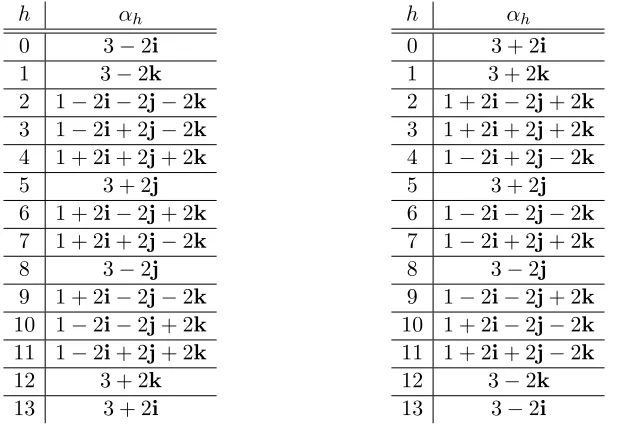
Example 6.4. Whenl= 13,we havea= 3, b= 2 ande= 8.The cases listed in (16) are no longer exhaustive. The correspondence is given in Table 2.
h αh
0 3−2i 1 3−2k 2 1−2i−2j−2k 3 1−2i+ 2j−2k 4 1 + 2i+ 2j+ 2k 5 3 + 2j 6 1 + 2i−2j+ 2k 7 1 + 2i+ 2j−2k 8 3−2j 9 1 + 2i−2j−2k 10 1−2i−2j+ 2k 11 1−2i+ 2j+ 2k 12 3 + 2k 13 3 + 2i
h αh
0 3 + 2i 1 3 + 2k 2 1 + 2i−2j+ 2k 3 1 + 2i+ 2j+ 2k 4 1−2i+ 2j−2k 5 3 + 2j 6 1−2i−2j−2k 7 1−2i+ 2j+ 2k 8 3−2j 9 1−2i−2j+ 2k 10 1 + 2i−2j−2k 11 1 + 2i+ 2j−2k 12 3−2k 13 3−2i
Table 2: The correspondence when∈8 + 13Z13 (left) and when ∈5 + 13Z13 (right).
7
Strong Approximation
In this section we briefly explain the significance of Strong Approximation to Ramanujan graphs and particularly the LPS graphs above. As discussed in Section 5 we may consider G(A), the adelic points of a linear algebraic groupGdefined over Q.The groupG(Q) embeds diagonally into G(A),and it is a discrete subgroup. The groups G(Qv) are also subgroups ofG(A),andG(A) has a well-defined projection onto G(Qv). Similarly, for a finite set of places S we may take GS, the
Strong Approximation (when it holds) is the statement that for a group G and a finite set of placesS the subgroupG(Q)GS isdense inG(A).This implies that
G(A) =G(Q)GSK for any open subgroup K ≤G(A). (21)
For example, Strong Approximation holds forG= SL2 and any set of placesS ={v}.However, in the form written above itdoes not hold for GL2 or PGL2.However one can prove results similar to (21) for GL2 adding restrictions on the subgroup K:
G(A) =G(Q)GSK for an open subgroup K≤G(A) ifK is “sufficiently large.” (22)
Here we shall have
K =Y
v /∈S
Kv; Kv ≤G(Zv) (23)
and the condition of being “sufficiently large” can be made precise by requiring that the determinant map det :Kv →Z×v be surjective for all v6∈S.
Strong Approximation holds for the algebraic group of elements of a quaternion algebra of unit norm [Vig80, Th´eor`eme 4.3]. We shall use this statement to prove a statement like (22) for the algebraic group of invertible quaternions. A similar statement then holds for G0 =B×/Z(B×) and a subgroupK0 that is not quite “large enough.” The implications for Pizer graphs and LPS graphs will be discussed in Sections 7.2 and 7.3 below.
These statements coming from Strong Approximation are crucial for proving that the various constructions produce Ramanujan graphs. As seen in Section 5 the Ramanujan property of a graph can be expressed in terms of its eigenvalues. Given a graph (constructed e.g. via local double cosets as seen above) the Strong Approximation theorem can be used to relate its spectrum to the representation theory of G(A). In that context a theorem of Deligne resolves the issue by proving a special case of the Ramanujan conjecture (see [Lub10, Theorem 6.1.2, Theorem A.1.2, Theorem A.2.14] and [Del71]).
7.1 Approximation for invertible quaternions
The argument below is adapted from [Gel75, Section 3] and [Lub10, 6.3].5
Let B be a (definite) quaternion algebra over Q, B× its invertible elements and B1 = {b ∈ B | N(b) = 1} its elements of reduced norm 1, recall N(b) = b¯b. Let l be a prime where B is split. Then by [Vig80, Th´eor`eme 4.3] we have thatB1(Q)B1(Ql) is dense in B1(A) thus B1(A) = B1(
Q)B1(Ql)K for any open subgroup K ≤B1(A).An open subgroupK ≤B1(A) is of the form K =Q
vKv whereKv ≤Bv1 is open and Kv =B1(Zv) for all but finitely many placesv.It follows
that given any open subgroups Kv(B1) ≤ B1(Zv) (v 6= l) such that K(B
1)
v = B1(Zv) for all but
finitely many places v we have that
B1(A) =B1(Q)B1(Ql)
Y
v6=l
Kv(B1). (24)
To make a similar statement for B× it will be necessary to impose a restriction on the open subgroups Kv.
5In fact, since at every split placevwe haveB×
(Qv)∼= GL2(Qv) with the reduced norm onB×corresponding to
Theorem 7.1. Let Kv ≤ B×(Zv) for every place l =6 v < ∞ so that Kv = B×(Zv) for all but
finitely many v, and the norm map N :Kv →Zv× is surjective for every place v. Then
B×(A) =B×(Q)B×(R)B×(Ql)
Y
l6=v<∞
Kv. (25)
Note that by [Voi18, Lemma 13.4.6] the norm map N :B×(Zv) → Zv× is surjective for every
nonarchimedeanv.
Proof. Let b ∈ B×(A), we need to show b is contained on the right-hand side. To write b as a product according to the right-hand side of (25) we shall use (24), strong approximation for B1. Observe first that it suffices to show that anyb∈B×(A) can be written as
b=rhk, wherer ∈B×(Q), h∈B1(A), and k∈B×(R)B×(Ql)
Y
l6=v<∞
Kv. (26)
This is because the intersectionsKv∩B1(Qv) are open subgroups ofB1(Zv) (andB×(Zv)∩B1(Zv) =
B1(Zv) at all but finitely many places). It thus follows from (24) (choosingK(B
1)
v :=Kv∩B1(Qv))
that the factorh∈B1(
A)⊆B×(A) from (26) is contained on the right-hand side of (25). It follows that thenb=rhk is contained on the right-hand side of (25) as well. (Note that here the factors of h andk belonging to different components B×(Qv) commute.)
So we must show that any b ∈B×(A) decomposes as in (26). Let b = (bv)v for bv ∈B×(Qv)
and setnv :=N(bv).For all but finitely many placesv we have bv ∈B×(Zv) and hencenv ∈Zv×.
At a finite set T of finite places we may writenv ∈vmvZv×.Let us take
nQ= Y
v∈T
vmv. (27)
ThennQ ∈Q>0, nQ ∈Zv× for everyv /∈T, v <∞and hence n−1
Q nv ∈Zv
× forevery finite placev. It is a fact that there is an r∈B×(Q) such that N(r) =nQ.Then for thisr we have that the norm ofr−1b∈B×(A) is in Zv× for every finite place v.
Let us write (r−1b)v for the component of r−1b ∈ B×(A) at a place v. There exists a k ∈
B×(R)B×(Ql)
Q
l6=v<∞Kv, k = (kv)v such that kl = (r−1b)l and k∞ = (r−1b)∞ and N(kv) =
N((r−1b)v) every other place. This follows from the fact that the norm map N : Kv → Zv× is
surjective.
Now let h =r−1bk−1.We show h ∈B1(A).Write h = (hv)v forhv ∈B×(Qv).It follows from
the choice of k that hl and h∞ are the identity element of B×(Ql) and B×(R) respectively, and N(hv) = 1 at every other place v. This implies that indeed h ∈B1(A). This completes the proof
that a decomposition as in (26) exists, and in turn the proof of (25).
7.2 Strong Approximation for LPS graphs
Section 6.3 that G0 is the Q-algebraic group B×/Z(B×).Let us fix the prime l ≡1 mod 4 as in Section 6. In a similar manner to the proof of (25) is follows that
G0(A) =G0(Q)G0(R)G0(Ql)
Y
l6=v<∞
G0(Zv). (28)
Recall that sinceBsplits atlwe haveG0(Ql)∼= PGL2(Ql).We wish to have a statement similar
to (28) above, replacingG0(Zv) atv= 2 andv =pby congruence subgroupsK20 andKp0.(Thispis
the one fixed above in Section 6.) Then isomorphism will no longer hold, but the right-hand side will be a finite index normal subgroup of G0(A).
The choice of the smaller subgroupsK20 and Kp0 is as follows. Forv∈ {2, p}let Kv0 = ker G0(Zv)→G0(Zv/vZv)
. (29)
Here Zv/vZv =Fv is a finite field, hence G0(Zv/vZv) is finite. It follows that the index [Kv :Kv0]
is finite. In fact since B2,∞ splits overp we have thatG0(Zp/vZp)∼= PGL2(Fp),hence [Kp :Kp0] =
p(p2−1).At v= 2 we have G0(F2) =B×(F2) hence [K2:K20] = 8.
Let us set Kv0 as above ifv ∈ {2, p}and Kv0 =Kv =G0(Zv) otherwise, and let us define
H2p:=
G0(Q)G0(R)G0(Ql) Y
l6=v<∞ Kv0
. (30)
By [Lub10, Proposition 6.3.3] Strong Approximation proves that H2p is a finite index normal
subgroup of G0(A).
From the definition of H2p in equation (30) we have a surjection from
G0(Ql)→G0(Q)\H2p/G0(R)
Y
l6=v<∞ Kv0.
If gl and gl0 ∈ G0(Ql) are mapped to the same coset on the right hand side then there exists
gq ∈ G0(Q), gr ∈ G0(R) and k = Ql6=v<∞kv ∈ Ql6=v<∞Kv0 such that gl = gqg0lgrk. This is
equivalent to saying gl = gqgl0 and gq ∈Kv0 for all l 6=v < ∞. By the definitions of the Kv0s this
last condition impliesgq ∈Γ(2p). Thus we see that
Γ(2p)\G0(Ql)/G0(Zl)∼=G0(Q)\H2p/G0(R)
Y
v<∞
Kv0. (31)
Strong approximation in the manner discussed above is used to prove that LPS graphs are Ramanujan. First one shows that the finite (l+ 1)-regular graph Γ(2p)\T is Ramanujan if and only if all irreducible infinite-dimensional unramified unitary representations of PGL2(Ql) that appear
in L2(P GL2(Ql)/Γ(2p)) are tempered [Lub10, Corollary 5.5.3]. Then by the isomorphism above
which follows from Strong Approximation, one can extend a representation ρ0l of PGL2(Ql) to an
automorphic representationρ0 ofG0(A) inL2(G0(Q)\G0(A)). By the Jacquet–Langlands correspon-dence, ρ0 corresponds to a cuspidal representation ρ of PGL2(A) in L2(PGL2(Q)\PGL2(A)) such thatρvis discrete series for allvwhereBramifies (so in our case, 2 and∞) [Lub10, Theorem 6.2.1].
Finally, Deligne has proved the Ramanujan–Peterson conjecture in this case of holomorphic mod-ular forms [Lub10, Theorem 6.1.2], [Del71], [Del74] which says that forρ a cuspidal representation of PGL2(A) inL2(PGL2(Q)\PGL2(A)) with ρ∞ discrete series,ρl is tempered [Lub10, Theorems
7.1.1 and 7.3.1]. Under the Jacquet–Langlands correspondence, the adjacency matrix of our graph X corresponds to the Hecke operator Tl [Lub10, 5.3] and the Ramanujan conjecture is equivalent
7.3 Strong Approximation for Pizer graphs
Now we turn to discussing how strong approximation is useful in establishing the bijections in (4). In Section 8 we will discuss Pizer’s construction of Ramanujan graphs. These graphs are isomorphic to supersingular isogeny graphs. Their vertex set is the class group of a maximal order O in the quaternion algebraBp,∞. This set is in bijection with an adelic double coset space, which in turn is in bijection with a set of local double cosets.
Let B = Bp,∞ be a quaternion algebra (over Q) ramified exactly at ∞ and at a finite prime p. At every finite prime v, B(Qv) has a unique maximal order up to conjugation [Vig80, Lemme
1.4]. Given a maximal orderO ofB,one may define the adelic group B×(Af) as a restricted direct
product of the groups B×(Qv) over the finite places, with respect to O×v.(Recall that this means
that any element of B×(Af) is a vector indexed by the finite places v; the component at v is in
B×(Qv) and in fact in O×v at all but finitely many places.) This adelic object does not in fact
depend on the choice of the maximal idealO.In particular, at any prime l6=p whereB splits we have B×(Ql)∼= GL2(Ql) and Ol×∼= GL2(Zl).
Let us now fix a primel whereB splits. The same argument as in Section 7.1 works restricted toB×(Af) (the finite ad`eles). It follows that we have
B×(Af) =B×(Q)B×(Ql)
Y
l6=v<∞
B×(Zv). (32)
Proposition 7.2. We have the bijections (cf. [CGL09, (1)])
B×(Q)\B×(Af)/
Y
v<∞
B×(Zv)∼=(O(Z[l−1]))×\B×(Ql)/B×(Zl)
∼
=(O(Z[l−1]))×\GL2(Ql)/GL2(Zl).
(33)
Proof. The first bijection follows from (32) and an argument similar to the proof of (31). Indeed, (32) implies that there is a surjection
B×(Ql)→B×(Q)\B×(Af)/
Y
l6=v<∞
B×(Zv). (34)
Now two elements gl, gl0 ∈ B×(Ql) land in the same double coset via this bijection if and only
if gl = gqgl0k in B×(Af). Then gl = gqgl0 (from equality at the place l) and gq ∈ B×(Zv) (from
equality at the places l 6= v < ∞). Consider the element gq ∈ B(Q), for example in terms of its coordinates in the standard basis{1,i,j,k} of B.Since gq∈B×(Zv) we have thatgq∈ O(Z[l−1]), and gq ∈ B×(Ql) implies that in fact gq ∈ (O(Z[l−1]))×. This completes the proof of the first
bijection in (33).
Now the second bijection follows from the fact thatB splits at the primeland henceB×(Ql)∼=
GL2(Ql) with the unique maximal order GL2(Zl).