Eleventh Floor, Menzies Building Monash University, Wellington Road CLAYTON Vic 3800 AUSTRALIA
Telephone: from overseas:
(03) 9905 2398, (03) 9905 5112 61 3 9905 2398 or 61 3 9905 5112
Fax:
(03) 9905 2426 61 3 9905 2426
e-mail: [email protected]
Internet home page: http//www.monash.edu.au/policy/
Reducing Illegal Migrants in the U.S.:
A Dynamic CGE Analysis
by
P
ETER
B.
DIXON
Centre of Policy Studies
Monash University
M
ARTIN
JOHNSON
U.S. Department of Commerce
AND
M
AUREEN
T.
RIMMER
Centre of Policy Studies
Monash University
General Paper No. G-183 July 2008
ISSN 1 031 9034 ISBN 0 7326 1590 9
Reducing illegal migrants in the U.S.: a dynamic CGE analysis by
Peter B. Dixon, Centre of Policy Studies, Monash University Martin Johnson, U.S. Department of Commerce
and
Maureen T. Rimmer, Centre of Policy Studies, Monash University
July 15, 2008
JEL codes: J61; C68.
Key words: Illegal immigration; dynamic modeling; U.S. immigration policy
Abstract
Contents
Summary
Acknowledgements
1. Introduction
2. The USAGE model and key macro assumptions
2.1. Production technologies and household preferences
2.2. Inflation
2.3. Investment and rates of return
2.4. Private and public consumption, and the public-sector deficit
3. The USAGE-M approach to modeling the labor market
3.1. Introduction
3.2. Workforce, categories, functions and activities
3.3. Labor supply from each category to each activity
3.4. Demand for labor in the U.S.
3.5. Relationship between after-tax and before-tax wage rates in the U.S.
3.6. Wage adjustment
3.7. The determination of everyone’s activity: who gets the jobs and
what happens to those who don’t?
4. Restricting the supply of foreign-illegal labor to the U.S.
4.1. Net and gross flows of illegal migrants into U.S. employment
4.2. Macroeconomic effects of reducing the supply of illegal migrants
4.3. Industry results
4.4. Occupational employment and wage effects for legal U.S. workers
4.5. Wage and employment results for foreign-illegal, foreign-legal and
domestic workers
4.6. Effects on aggregate welfare of legal U.S. residents
5. Restricting the demand for foreign-illegal labor in the U.S. by taxes on employers
6. Sensitivity analysis
6.1. Restricting the demand for foreign-illegal labor in the U.S. by
punitive measures on employers
6.2. Varying provision of public services to illegal migrants
6.3. Varying the size of the reduction in foreign-illegal employment
6.4. Varying key demand parameters
6.5. Varying the key supply parameter
7. Concluding remarks
Acknowledgements
The work reported in this paper is part of a larger project concerned with the development and application of the USAGE model of the U.S. economy. Since its inception in 2001, the USAGE project has been guided and inspired by Bob Koopman. Without his support, the USAGE model would not exist.
Summary
(1) We use the USAGE-M model to simulate the effects on the U.S. economy of policies to restrict the employment of illegal migrants. A USAGE-M simulation consists of two runs: a basecase forecast run incorporating business-as-usual assumptions, and a policy run incorporating the policy under analysis. By comparing the results from the two runs, we generate the effects of the policy as percentage deviations in variables of interest away from their basecase forecast values.
(2) In our basecase forecast, employment of foreign illegal workers grows from 7.3m in 2005 to 12.4m in 2019, an annual rate of growth of 3.8%. Rapid growth of illegal employment occurs despite only moderate growth (about 1% a year) in the net inflow of illegal migrants. The reason is that net inflow in 2005 was large, so that even if there were no growth in net inflow, the stock of illegal workers in the U.S. would increase rapidly. By contrast with the 3.8% annual growth in employment of illegal workers, employment of legal workers grows at an annual rate of only 1%.
(3) We analyze two types of programs to lower the number of illegal migrants in U.S. employment:
a. Simulation SR: restricting supply by increasing the costs to illegal migrants of migrating to the U.S. (increased border security, higher smugglers fees, deportation, improved conditions in “Mexico”);
b. Simulation DR: restricting demand by increasing the costs of employing illegal migrants (taxes, fines).
(4) The SR and DR simulations are scaled to have the same long-run effect on foreign-illegal employment. The policy shocks in both simulations cause employment of illegal migrants to be 28.6% less in 2019 than it otherwise would have been, that is they generate deviations of -28.6%. This reduces the average annual growth of illegal employment between 2005 and 2019 from the basecase level of 3.8% to 1.4%. The paper provides guidance on how to deduce from the SR and DR results the effects of policies of different scale.
(5) With 28.6% cent fewer illegal workers, both simulations show negative deviations in the size of the economy in 2019 of about 1.6 %. Applied to the GDP of 2007, this is about $200 billion.
(6) The adjustment to a smaller economy would require a period in which the investment share in U.S. GDP was significantly weaker than it otherwise would have been. Both simulations show strong negative deviations in the early years for the I/GDP ratio. (7) During the period of weak investment, both simulations show negative deviations in
the exchange rate with consequent positive deviations in exports and negative deviations in imports.
(8) With the cut in illegal employment, both simulations show the expenditure
components of GDP settling in the long run to levels between 0.8 and 2.7 per cent lower than they otherwise would have been.
(10) Macro, industry and occupational effects are quite similar in the two simulations, indicating that these effects are insensitive to the type of program used to lower illegal employment.
(11) Industry effects mainly reflect macro results. An industry’s current reliance on foreign illegal workers is relatively unimportant. Our results show industries with high reliance on foreign-illegal labor that perform relatively well in our simulations and others that perform relatively poorly. Ground maintenance and construction both have high reliance. Ground maintenance does relatively well because of its
connection with private and public consumption. Construction does poorly because of its connection with investment. Similarly, our results show industries with low reliance on foreign-illegal labor that perform relatively poorly and others that perform relatively well. Machinery and Utilities both have low reliance. Machinery does relatively poorly because of its connection with exports and investment. Utilities does well because of its connection with consumption.
(12) The programs increase jobs for domestic workers in the type of work performed by illegal migrants (e.g. construction laborers, drywall installers, miscellaneous agricultural workers, grounds maintenance workers, cooks, etc).
(13) Measuring welfare by public and private consumption, we find that the legal
population (domestic and legal migrant) are worse off under the programs. In the SR simulation, the loss in private and public consumption for the legal population is 0.52 per cent in 2019. Applied to private and public consumption of 2007, this is about $60 billion. In the DR simulation, the loss in consumption for the legal population is 0.08 per cent in 2019, or about $9 billion in 2007 equivalent terms.
(14) The main negative effect on the legal population from a reduction in employment of foreign-illegal workers is that it increases the share of legal workers in low-wage occupations. We refer to this as the occupational-mix effect.
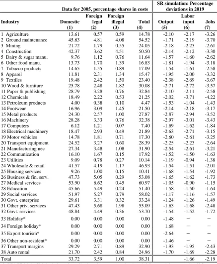
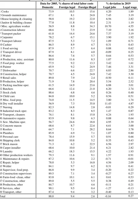
(15) The type of program matters for the welfare effect. Demand-reducing taxation of illegal migrant employment (Simulation DR) is less damaging to the legal population than supply-reducing increases in the costs to illegal workers of entering the U.S (Simulation SR). The principal reason is illustrated by what we call Borjas diagrams, showing demand and supply curves for illegal labor. These diagrams demonstrate that both programs increase the cost per unit of foreign-illegal labor to employers. Supply-restricting programs allow the foreign-illegal employees who remain in the U.S. to capture the increase in cost as an increase in their wage rate.
Demand-contracting programs, implemented by taxes and fines, transfer all of the cost increase (and more) to the U.S. Treasury.
(16) The advantage of the DR over the SR approach depends crucially on our assumption that the DR policy is implemented as a pure transfer of money from employers of illegal migrants to the U.S. Treasury, a transfer does not involve dissipation of resources (capital and labor) by the employer. In a sensitivity simulation, we assume that demand restriction is implemented by criminal prosecutions and business
(17) In both the SR and DR simulations we assume that public consumption per capita devoted to illegal migrants and their dependents in the U.S. is 49% of that devoted to legal residents. In a sensitivity simulation, we increase this percentage to 71%. Despite the prominence of the public expenditure issue in political discussions of illegal migrants, we find that this variation in the public expenditure assumption has only a minor impact on the welfare results for legal residents.
(18) The effects of supply restriction are approximately proportional to the size of the program. A supply-restriction program that reduces long-run employment of illegal migrants in the U.S. by 57.2% has approximately twice as large an effect on all variables, including the welfare of legal residents, as a program that reduces long-run employment of illegal migrants by 28.6%.
(19) The welfare effect on legal residents of a demand restriction program implemented by taxes and fines responds in a non-linear way to the size of the program. For a small program, for example one that reduces illegal employment in the long-run by 14.3%, the favorable effects generated from the suppression of illegal wage rates outweigh the unfavorable efficiency effects of losing workers whose marginal products exceed their wage rates. For a large program, for example one that reduces illegal
employment in the long-run by 57.2%, the unfavorable efficiency effects outweigh the favorable wage-rate effects.
(20) For both SR and DR programs of a given size, large variations in the USAGE-M parameters controlling the elasticity of demand by U.S. employers for illegal workers have relatively little effect on the welfare results for legal residents.
(21) Similarly, large variations in parameters controlling the elasticity of supply to U.S. employers of illegal workers have relatively little effect on the welfare results for legal residents.
(22) USAGE-M identifies six factors that determine the welfare result for legal residents of programs to restrict employment of illegal migrants:
1. Borjas effects covering changes in producer surplus via efficiency triangles and wage rectangles;
2. effects on the skill composition of legal employment (occupation-mix);
3. capital effects encompassing long-run changes in the wealth of legal residents and effects on taxes collected from capital owned by foreigners;
4. effects on aggregate employment of legal residents; 5. public expenditure effects; and
6. effects on the U.S. terms of trade.
The reason for the relative insensitivity of the welfare result for legal residents to changes in demand and supply parameters is that these changes impinge on only the first of the six factors.
(23) The calculations in this paper do not incorporate the costs of implementing polices, that is the administrative costs of imposing taxes and fines, prosecuting employers and enhancing border security.
1. Introduction
There are about 7.5 million illegal migrants working in the U.S., accounting for nearly 5 per cent of total employment. These are people who have entered the U.S illegally, mainly from Mexico or other parts of Latin America, or who have stayed in the U.S. beyond the expiry date on their visas.
Public attitudes in the U.S. to the illegal migrants vary across a wide spectrum, from the view that they are impoverishing poorer legal residents by depriving them of jobs to the view that they are a vital part of the U.S. economy because they perform tasks that legal residents are not willing to undertake. The illegal migrant issue is now a major component of the political debate with policy suggestions ranging from mass deportation to legalization and amnesty.
This paper provides some quantitative analysis that we hope will be helpful in informing policy discussions. We project the effects:
• on macroeconomic variables including GDP, aggregate employment, capital stock, exports, imports, investment and public and private consumption;
• on employment and wage rates by occupation for legal residents;
• on outputs and employment of industries; and
• on the overall welfare of legal residents;
of two broad approaches to reducing employment of illegal migrants. The first approach is to cut supply through tighter border security, deportation or other policies that reduce the desirability to potential illegal migrants of working in the U.S. The second approach is to cut demand through taxes and fines imposed on of employers of illegal migrants or through criminal prosecutions of these employers.
In making our projections, we use USAGE1, a detailed, dynamic CGE model of the U.S. economy. For the present project, we create a labor-market-extended version of USAGE, called USAGE-M. In this extension, we disaggregate the demand for labor by each industry into demands for workers classified by birth place (domestic and foreign), legal status (legal and illegal) and occupation (50 occupations emphasizing those in which illegal migrants are predominantly employed. We also disaggregate the supply side of the labor market into supplies by workers classified by birth place, legal status and recent labor-market function including working outside the U.S.
The paper is organized as follows. Section 2 describes the USAGE model and our main macro assumptions. Section 3 sets out the labor-market extension. This section is technical and can be skipped by readers who are not concerned with implementation details. All principal results in later sections are explained by back-of-the-envelope calculations incorporating familiar economic mechanisms that can be understood independently of section 3. Sections 4 and 5 describe and explain our simulations of supply restriction (the SR simulation) and demand restriction (the DR simulation). Section 6 presents sensitivity analysis covering the effects on our main results of changes in assumption concerning:
• resource costs imposed on employers by demand-side policies;
• provision of public services to illegal migrants and their families;
• the scale of programs to restrict the employment of illegal migrants;
• key parameters determining the elasticity of demand by U.S. employers for the services of illegal migrants with respect to their wage rate; and
1
• key parameters determining the elasticity of supply to U.S. employers of illegal workers with respect to their wage rate.
Concluding remarks and suggestions for future research are in section 7.
2. The USAGE model and key macro assumptions
USAGE is a detailed, dynamic CGE model of the U.S. It has been developed at the Centre of Policy Studies, Monash University, in collaboration with the U.S. International Trade Commission.2 The theoretical structure of USAGE is similar to that of the MONASH model of Australia (Dixon and Rimmer, 2002). However, in both its theoretical and empirical detail, USAGE goes beyond MONASH. USAGE can be run with up to 500 industries, 700 occupations and 51 regions (50 States plus the District of Columbia). While the standard version of USAGE contains considerable detail, we often find that further detail must be added to capture the essence of the issue under consideration. For this paper, we created a new version of USAGE with a labor-market-extension (section 3) designed to facilitate the analysis of issues concerning illegal migrants. This version is referred to as USAGE-M. It is implemented with 38 industries and 51 occupations. The first 50 occupations refer to jobs in the U.S. These occupations are chosen to retain maximum detail for activities in which illegal migrants are heavily employed. The 51st occupation is employment in the source countries for illegal migrants (e.g. Mexico). Inclusion of this occupation facilitates our modeling of inflows and outflows of illegal migrants.
USAGE includes three types of dynamic mechanisms: capital accumulation; liability accumulation; and lagged adjustment processes. Capital accumulation is specified separately for each industry. An industry’s capital stock at the start of year t+1 is its capital at the start of year t plus its investment during year t minus depreciation. Investment during year t is determined as a positive function of the expected rate of return on the industry’s capital. Expected rates of return can be determined by rational expectations (forward-looking) or static expectations in which only information from year t and earlier years is used.3 Liability accumulation is specified for the public sector and for the foreign accounts. Public sector liability at the start of year t+1 is public sector liability at the start of year t plus the public sector deficit incurred during year t. Net foreign liabilities at the start of year t+1 are specified as net foreign liabilities at the start of year t plus the current account deficit in year t plus the effects of revaluations of assets and liabilities caused by changes in price levels and the exchange rate. Lagged adjustment processes are specified for the response of wage rates to gaps between the demand for and the supply of labor by occupation. There are also lagged adjustment processes in USAGE for the response of foreign demand for U.S. exports to changes in their foreign-currency prices.
In a USAGE simulation of the effects of policy and other shocks, we need two runs of the model: a basecase or business-as-usual run and a policy run. The basecase is intended to be a plausible forecast while the policy run generates deviations away from the basecase caused by the policy under consideration. The basecase incorporates trends in industry technologies, household preferences and trade and demographic variables. These trends are estimated largely on the basis of results from historical runs in which USAGE is forced to track a piece of history. Most macro variables are exogenous in the basecase so that their paths can be set in accordance with forecasts made by expert macro forecasting groups such as the Congressional Budget Office. This requires endogenization of various macro
2
Prominent applications of USAGE by the U.S. International Trade Commission include USITC (2004 and 2007).
3
propensities, e.g. the average propensity to consume. These propensities must be allowed to adjust in the basecase run to accommodate the exogenous paths for the macro variables.
The policy run in a USAGE study is normally conducted with a different closure (choice of exogenous variables) from that used in the basecase. In the policy run, macro variables must be endogenous: we want to know how they are affected by the policy. Correspondingly, macro propensities are exogenized and given the values they had in the basecase. More generally, all exogenous variables in the policy run have the values they had in the basecase, either endogenously or exogenously, with the exception of the policy variables of interest. Comparison of results from the policy and basecase runs then gives the effects of moving the policy variables of interest away from their basecase values. In the analyses in sections 4 and 5, the basecase and policy runs differ with regard to the values given to exogenous variables representing the costs to illegal migrants of coming to the U.S. and the costs to U.S. businesses of employing illegal migrants. We interpret the differences between the results in the basecase and the policy runs as the effects of policies that increase the obstacles faced at U.S. borders by potential illegal migrants and the effects of policies that impose fines and taxes on U.S. employers of illegal migrants.
In USAGE-based policy analyses, the policy closure introduces important background macroeconomic assumptions. Labor-market aspects of the assumptions introduced into the simulations reported in sections 4 and 5 are discussed in section 3. Other features of our policy closure and the corresponding macroeconomic assumptions are as follows.
2.1. Production technologies and household preferences
USAGE contains variables describing: primary-factor and intermediate-input-saving technical change in current production; input-saving technical change in capital creation; input-saving technical change in the provision of margin services; and input-saving changes in household preferences. In the policy runs described in sections 4 and 5, all of these variables are exogenous and kept on their basecase paths. Thus we assume that changes in immigration policy have no effect on technology or household preferences.
2.2. Inflation
In our policy closure, the price deflator for GDP is exogenous and set on its basecase path. Thus we assume that changes in immigration policy have no effect on inflation. Underlying this assumption is the idea that the Federal Reserve adjusts monetary policy to achieve a given inflation target.
2.3. Investment and rates of return
For this paper, the policy closure is set so that expected rates of return are generated by projecting current information. This is convenient because it allows the model to be solved recursively (in a sequence, one year at a time). We do not consider that the alternative, rational expectations, would add realism.
2.4. Private and public consumption, and the public-sector deficit
In our policy closure, the average propensities for legal residents and illegal migrants to undertake private consumption out of household disposable income are exogenous. We set them on their basecase paths. Thus we assume that these propensities are not affected by immigration policy. In the case of illegal migrants, we assume that their savings are remitted to their home countries.4 Consequently, our policy runs capture the effects on the current account of reduced remittances associated reduced employment of illegal migrants. In determining public consumption expenditure in our policy runs, we use the equation:
CPRIV(leg) CPRIV(leg)
CPUB F * * N(leg) * F * * N(ill)
N(leg) N(leg)
⎡ ⎤
⎛ ⎞ ⎛ ⎞
= ⎜ ⎟ + α ⎢ ⎜ ⎟⎥
⎝ ⎠ ⎣ ⎝ ⎠⎦ (2.1)
where
CPUB is the volume of public consumption;
CPRIV(leg) is private consumption by legal residents ;
N(ill) is the number of people in the U.S. in illegal migrant families (which we will call for convenience the number of illegal people);
N(leg) is the number of people in the U.S. in legal resident families (which we will call for convenience the number of legal people);
α is a parameter; and F is a shift variable.
In the basecase run, F is endogenous and adjusts to make (2.1) compatible with extraneous forecasts for the path of public consumption (CPUB). In the policy closure, F is exogenous and is set on its basecase path. With F exogenous, (2.1) generates deviations in public consumption away from its basecase path as the sum of deviations in two components. The first component is public consumption devoted to legal people. We assume that as legal people become richer, they demand more public services. In particular we assume that public consumption devoted to each legal person is proportional to private consumption per legal person. The second component is public consumption devoted to illegal people. We assume that public consumption per capita devoted to illegal people is proportional to that devoted to legal people. Under this assumption, illegal people cannot be prevented from enjoying improvements in public amenities made available for legal people.
Our central estimate for the factor of proportionality, α, is 0.49.5 The main source for this estimation was Rector and Kim (2007)6. They provide detailed estimates by function (education, health etc) of government expenditures on households headed by low-skilled immigrants (those without a high school degree). We used these estimates as a starting point for calculating government expenditures on households headed by illegal immigrants. In doing this we recognized that not all government services available to legal migrants are available to illegal migrants. Thus, for example, in estimating education
4
This assumption could be modified if we had data to suggest that not all of savings by illegal migrants are remitted. However, our remittance assumption is not important in determining the principal results in sections 4 to 6. If we assumed that illegal migrants kept their savings in the U.S., then our results would indicate increased ownership of U.S. assets by illegal migrants offset by reduced ownership by foreigners from outside the U.S. There would be little effect on our welfare results for legal residents.
5
Subsection 6.2 reports the effects of varying α. 6
expenditures on illegal migrant households, we assumed that these are the same per child at the primary and secondary level as for low-skill migrant households. At the tertiary level we assumed zero government expenditure on illegal migrants. This is because very few states allow illegal migrants to enroll in public-sector tertiary institutions. For pure public goods such as defense, we assumed that illegal migrants have no effect on expenditure.
On the income-side of the public-sector budget, we assume in our policy runs that tax rates adjust to ensure that the public sector deficit follows its basecase path.
3. The USAGE-M approach to modeling the labor market
3.1. Introduction
The six key ingredients in the labor market specification of USAGE-M are: (1) the division of the workforce into categories at start of each year reflecting
workforce functions in the previous year;
(2) the identification of workforce activities, that is what people do during the year; (3) the determination of labor supply from each category to each activity;
(4) the determination of demand for labor in employment activities;
(5) the specification of wage adjustment processes reflecting demand and supply; and (6) the determination of everyone’s activity: who gets the jobs and what happens to
those who don’t?
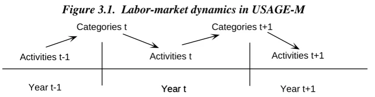
A broad picture of the specification can be obtained from Figure 3.1. We divide the workforce at the start of year t into categories. These categories reflect the activities that people undertook in year t-1, with the main activities being employment in occupations. The activities that people in a given category undertake in year t are determined mainly by their supply to that activity, relative to supply from people in other categories, and by demand for the services of that activity.
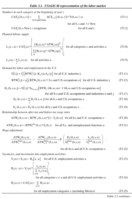
Table 3.1 lists the equations explained in this section that form the labor-market module of USAGE-M.
3.2. Workforce, categories, functions and activities
We adopt two concepts of workforce: the U.S. workforce and the extended workforce. The U.S. workforce is everyone of working age in the U.S excluding people in full time education and those who are ruled out of work by disabilities. Under this definition, the U.S. workforce includes discouraged workers and other people who are not actively seeking employment. The extended workforce is the U.S. workforce plus potential foreign illegal migrants working outside the U.S. For convenience we refer to these potential foreign illegal migrants as working in Mexico.
At the beginning of each year, we allocate people in the extended workforce to categories according to their birthplace, legal status and recent labor market function. We allow for two birthplaces, domestic7 and foreign, and two legal statuses, legal and illegal. All people with birthplace “domestic” have the status “legal”. Some foreign residents of the U.S. are legal while others are illegal. We classify all workers in Mexico as illegal. This of course does not mean that Mexicans are working illegally in Mexico. It means that from the point of view of the U.S., Mexican workers in Mexico are potential foreign illegal migrants.
7
Table 3.1. USAGE-M representation of the labor market
Numbers in each category at the beginning of year t
(
)
(
)
t t 1
ss Legal status
CAT (b, s, ) ACT− (b, ss, ) * T(b, ss, , s) ∈
= ∑
A A A (T3.1)
for all b, s and A≠New
t
CAT (b, s, New)=exogenous for all b and s . (T3.2) Planned labour supply
(
)
(
)
t t t t t t qB (c; a) * ATW (a) L (c ; a) CAT (c) *
B (c; q) * ATW (q) η η ⎡ ⎤ ⎢ ⎥ ⎢ ⎥ = ⎢ ⎥ ∑ ⎢ ⎥ ⎢ ⎥ ⎣ ⎦
for all categories c and activities a (T3.8)
t t
c
L (a)= ∑L (c; a) for all activities a . (T3.9) Demand for labor and employment in the U.S.
(
)
1 1 1
t j t t t
D ( j)=f BTW ( j) ; K ( j); A ( j) for all U.S. industries j (T3.11)
(
)
1 1
t j t
BTW ( j)=g BTW (b, s, o)∀b, s and U.S. occupations o for all U.S. industries j (T3.12)
(
)
1
t t b,s,o, j t
D (b, s, o, j)=D ( j) * h BTW (bb, ss, oo) ∀bb, ss and U.S. occupations oo
for all b,s and U.S. occupations and industries o and j (T3.17)
t t
j
D (b, s, o)= ∑D (b, s, o, j) for all b, s and U.S. occupations o . (T3.18)
t t
E (b, s, o)=D (b, s, o) for all b, s and U.S. occupations o . (T3.19) Relationship between after-tax and before-tax wage rates
(
)
t t t
ATW (b, s, o)=BTW (b, s, o) * 1 T (b, s)− for all b,s and U.S. occupations o (T3.20)
ave
t t t
ATW (b, s, u)=BTW (b, s) * F (b, s) for all b,s and unemployment functions u (T3.21) Wage adjustment
t t 1 t t
base base base base
t t 1 t t
ATW (b, s, o) ATW (b, s, o) D (b, s, o) L (b, s, o)
ATW (b, s, o) ATW (b, s, o) D (b, s, o) L (b, s, o) − − ⎛ ⎞ ⎜ ⎟ − = β − ⎜ ⎟ ⎝ ⎠ ,
for all (b,s) and all U.S. occupations o (T3.22) Vacancies, and movements into employment activities
[
]
t t t
V (a)=E (a) H a ; a− for all U.S. employment activities a (T3.23)
t
t t
t s a
L (c; a) H (c ; a) V (a) *
L (s; a) ≠ ⎡ ⎤ ⎢ ⎥ = ⎢ ⎥ ∑ ⎢ ⎥ ⎣ ⎦ ,
for all categories c ≠ a and all U.S. employment activities a. (T3.24)
t t t
a c H (c; c) CAT (c) H (c; a)
≠
= − ∑ ,
Table 3.1 continued
Movements into unemployment and Mexican activities
c t
t
L (c; u) (c) * CAT (c) for short run unemployment activities u H (c; u)
0 for long run unemployment activities u
+ μ −
⎧
= ⎨ −
⎩
for all U.S. employment categories c , (T3.26)
a employment activ
t t t
0 for short run unemployment activities u H (c; u) CAT (c) H (c; a) for long run unemployment activities u
∈
− ⎧⎪
= ⎨ − ∑ −
⎪⎩
for all U.S. unemployment categories c and all unemployment activities u (T3.27)
a U.S. employ activ a U.S. employ activ
t t
t t t
CAT (c) H (c; a) for c not foreign, illegal and for short run unemploy activ u H (c; u) CAT (c) H (c; a) for c foreign, illegal and for Mexican activities u
0 otherwise ∈ ∈ − − ⎧ ∑ ⎪ ⎪ =⎨ − ∑ ⎪ ⎪⎩
for all New categories c and all unemployment or Mexican activities u . (T3.28)
a U.S. employ activ t
t t t
L (c; u) for c non Mexican H (c; u) CAT (c) H (c; a) for c Mexican
∈
− ⎧⎪
= ⎨ − ∑
⎪⎩
for all non-New categories c and for Mexican activities u (T3.29)
t t
c
H (c, a)=E (a)
∑ , for all U.S. unemployment activities and Mexican activities a (T3.30) Notation
(
)
t
CAT (b, s, )A is the number of people at the start of year t who are from birthplace b, have legal status s and who performed workforce function A in year t-1.
(
)
t
CAT (b, s, New) is the number of people at the start of year t who are from birthplace b, have legal status s and were not in the extended workforce in year t-1.
(
)
t 1
ACT− (bb, ss, )A is the number of people in activity (bb, ss, )A in year t-1.
T(b, ss, , s)A is the proportion of people in activity (b, ss, )A in year t-1 who are allocated to category
(b, s, )A at the start of year t.
t
L (c; a) is the labor supply that people in category c make to activity a. Both c and a are (b, s, )A triples.
t
L (a) is total labor supply to activity a.
base t
L (a) is the base or forecast value of L (a)t .
β is a positive parameter.
t
ATW (a) is the real after-tax wage rate of labor in activity a (for non-employment activities it is a social security payment or other support).
base t
ATW (a) is the base or forecast value of ATW (a)t .
η is a parameter reflecting the ease with which people feel that they can shift between activities.
t
B (c; a) is a variable reflecting the preference of people in category c for earning money in activity a in year t.
t
K ( j) is industry j’s capital stock.
1 t
BTW ( j) is the overall real before-tax wage rate to the industry.
t
A ( j) is a vector of variables that influence industry j’s demand for labor.
1 t
D ( j)is labor input to industry j.
Table 3.1 continued
t
BTW (b, s, o) is the real before-tax wage rate of workers of birthplace b, legal status s and U.S. occupation o.
t
D (b, s, o, j) is j’s input of labor of birthplace b, legal status s and U.S. occupation o.
t
D (b, s, o) is aggregate demand for (b,s,o) labor.
base t
D (b, s, o) is the base or forecast value of D (b, s, o)t .
t
E (b, s, o) is employment of (b,s,o) labor.
t
T (b, s) is the payroll and income-tax rate applying to all (b,s) workers in the U.S.
ave t
BTW (b, s) is the average real before-tax wage rate of (b,s) workers in the U.S.
t
F (b, s) is the fraction of BTWtave(b, s) that (b,s) people receive in unemployment activities from social security payments or other support.
t
V (a) is vacancies in activity a.
[ ]
tH c ; a is the flow of people from category c to activity a.
μ(c) is the fraction of people of category c people who become involuntarily unemployed.
Figure 3.1. Labor-market dynamics in USAGE-M
Year t-1 Year t Year t+1
Activities t-1 Activities t Activities t+1
Year t
Categories t Categories t+1
A person’s recent workforce function refers to what he or she did in the labor market in the previous year, year t-1. The functions we identify are:
employed in occupation m, where m is one of the 50 U.S. occupations identified in USAGE-M;
short-run unemployed in the U.S., that is unemployed for a substantial amount of year t-1 but not unemployed in year t-2;
long-run unemployed in the U.S., that is unemployed for a substantial amount of year t-1 and also of year t-2;
living in the U.S. but not in the workforce;
employed in the single Mexican occupation recognized in USAGE-M; living in Mexico but not in the workforce.
A final concept that we need to explain before setting out the algebra of the labor-market specification is activity. Activities are defined by birthplace, legal status and workforce function in the current year. Examples of activities in year t are: working in the U.S. as a domestic-legal construction laborer; working in the U.S. as a foreign-illegal cook; and experiencing short-run unemployment in the U.S. as a foreign legal resident. Another activity is working as a foreign illegal in Mexico. As already mentioned, we do not wish to imply that Mexicans are working illegally in Mexico. As we will see, Mexican workers in Mexico will be modeled as potential entrants to foreign illegal work activities in the U.S.
(
)
(
)
t t 1
ss Legalstatus
CAT (b, s, ) ACT− (b, ss, ) * T(b, ss, , s)
∈
= ∑
A A A (3.1)
for all b, s and non-new functions, i.e. A≠New
(
)
t
CAT (b,s, New) =exogenous for all b and s . (3.2)
In these equations,
(
)
t
CAT (b, s, )A is the number of people at the start of year t who are from birthplace
b, have legal status s and who performed workforce function A in year t-1.
(
)
t
CAT (b,s, New) is the number of people at the start of year t who are from
birthplace b, have legal status s and were not in the extended workforce in year t-1, that is the number of new (b,s) entrants to the extended workforce. If b is domestic and s is legal, then we have in mind high school and college graduates entering the job market in the U.S. If b is foreign and s is legal, then we have in mind newly admitted legal migrants of working age. If b is foreign and s is illegal, then we have in mind high school and college graduates entering the workforce in Mexico. There is no-one in the category domestic-illegal-new. As indicated in (3.2), the numbers of people in “New” categories is set exogenously, reflecting demographic factors.
(
)
t 1
ACT− (bb, ss, )A is the number of people in activity (bb,ss, )A in year t-1, that is
the number of people who, in year t-1, belonged to birthplace bb, had legal status ss and labor-force function A.
T(b,ss, ,s)A is the proportion of people in activity (b, ss, )A in year t-1 who are allocated to category (b, s, )A at the start of year t: we assume that people never change their birthplace.8
In the simulations reported in sections 4 and 5
,
we set0.99 for all and b, and for all s,ss such that s ss T(b, ss, ,s)
0.00 otherwise
= ⎧
= ⎨ ⎩
A A
. (3.3) Under (3.3), we assume that no-one changes legal status, and that one per cent of people in every activity in year t-1 drop out of the extended workforce at the beginning of year t, either through retirement or death. More sophisticated transition assumptions are possible. To allow for legalization of some foreign illegals in the U.S. and for differences in retirement/death rates across activities, we could set T(b, ss, , s)A according to:
T(b, ss, , s)A =Survive(b, ss, ) * P(s ss, )A A (3.4)
where
Survive(b, ss, )A is the proportion of people in activity (b,ss, )A in year t-1 who remain in the extended workforce in year t; and
P(s ss, )A is the probability of a surviving person who had legal status ss and
workforce function A in year t-1 achieving legal status s at the start of year t.
8
In (3.4), we continue to assume that people cannot change their birthplace but we allow for the possibility of changes in legal status. In future research we could investigate the implications of legalization programs by simulating the effects of suitable shocks to
P(s ss, )A for ss= illegal, s = legal and A≠Mexico.
3.3. Labor supply from each category to each activity
USAGE-M specifies labor supply from people in each category to each activity. Via these specifications, we ensure that people in a category with birthplace b and legal status s make offers only to activities with these characteristics. Thus, people in the category domestic-legal construction laborer can offer only to activities with the domestic and legal characteristics. Most of these people offer to the activity domestic-legal construction laborer, that is they offer to continue their employment of last year. However, some will offer to change occupation in response to changes in relative wages and a few will offer to unemployment. Some people in the category illegal Mexico will offer to foreign-illegal occupations in the U.S., that is they will seek to enter the U.S. as foreign-illegal migrants, and some people in foreign-illegal categories operating in the U.S. will make offers to the activity foreign-illegal Mexico, that is they will offer to return home. In making these decisions, people in these foreign-illegal categories compare wages in Mexico with wages for foreign-illegal occupations in the U.S.
In developing the labor-supply functions for USAGE-M, we assume that at the beginning of year t, people in category c [where c is a (birthplace, legal status, function) triple] decide their offers to activity a [where a is also a (b,s,A) triple] for the year by solving a problem of the form: choose Lt(c;a), for all activities a
to maximize U ATW (a) * L (c; a)c
[
t t ∀activities a]
(3.5)subject to t t
a
L (c; a)=CAT (c)
∑ (3.6)
where
Lt(c;a) is the labor supply that people in category c make to activity a;
CATt(c) is the number of people in category c;
ATWt(a) is the real after-tax wage rate of labor in activity a (for non-employment
activities, that is short-and long-run unemployment, ATWt(a) can be thought of as a
social security payment or other support); and
Uc is a homothetic function with the usual properties of utility functions (positive first
derivatives and quasi-concavity).
In (3.5) and (3.6), people in category c treat dollars earned in different activities as imperfect substitutes. This is a convenient and flexible specification through which we can allow labor supplies to shift between activities in response to changes in after-tax rewards. By specifying a separate utility function for each c, we can ensure that each category makes supplies to activities that are compatible with the category’s birthplace, legal status and occupational characteristics.
In the application presented in sections 4 and 5, Uc has the CES form:
(
)
1
1
c t t t
a
U B (c; a) * ATW (a) * L (c; a)
+η η
η +η
⎡ ⎤
⎢ ⎥
= ∑⎢ ⎥
⎢ ⎥
⎣ ⎦
where
η is a parameter reflecting the ease with which people feel that they can shift between activities; and
Bt(c;a) is a variable reflecting the preference of people in category c for earning money in activity a in year t.
The Bt(c;a)’s play two roles in our analysis. The first is via their initial settings, that is the values assigned to them in the base year, 2004, data.
• By setting B2004(c;a) at 0 if the birthplace and legal characteristics of c differ from those of a, we ensure that people in categories with birthplace b and legal status s offer labor only to (b,s) activities.
• By setting B2004(c;a) at relatively high values when c and a agree in their (b,s) characteristics and have a functional characteristic referring to the same occupation, we ensure that most people employed in year t-1 in occupation m (including the Mexican occupation) offer to continue to work in m in year t.
• By setting B2004(c;a) at suitably chosen positive values when c and a agree in their (b,s) characteristics but have functional characteristics referring to different occupations, we ensure that people make offers to work in occupations compatible with their skills.
• By setting B2004(c;a) at zero where the functional characteristic of c is either short-run or long-short-run unemployment and the functional characteristic of a is short-short-run unemployment, we ensure that no-one can stay in short-run unemployment in successive years or move from long-run unemployment back to short-run unemployment.
• By setting B2004(c;a) at a moderately large value where c and a agree in their (b,s) characteristics and c has the functional characteristic of short-run unemployment and a has the functional characteristic long-run unemployment, we introduce a mild discouraged-worker effect for people suffering short-run unemployment.
• By setting B2004(c;a) at a larger value where c and a agree in their (b,s) characteristics and where c and a both have the functional characteristic of long-run unemployment, we introduce a stronger discouraged-worker effect for the long-run unemployed.
The second role of the Bt(c;a)’s is to carry shocks in policy runs. In section 4, we represent the impact of tighter border security by reductions in the Bt(c;a)’s where c and a both have the (b,s) characteristics foreign illegal and c has the functional characteristics of either Mexico or New and a has the functional characteristic of a U.S. occupation.
Under (3.7), problem (3.5) - (3.6) generates labor-supply functions of the form:
(
)
(
)
t t
t t
t t
q
B (c; a) * ATW (a)
L (c ; a) CAT (c) *
B (c; q) * ATW (q)
η
η
⎡ ⎤
⎢ ⎥
⎢ ⎥
=
⎢∑ ⎥
⎢ ⎥
⎣ ⎦
. (3.8)
Total supply of labor to activity a is obtained as
t t
c
(
t) (
t)
ave ave
t(c ; a)=cat (c)t + η* atw (a) atwt − (c) + η* b (a) bt − (c)
A . (3.10)
In (3.10), the lowercase symbols At(c ; a), cat (c ) , atwt t(a) and bt(a) are percentage changes in the variables denoted by the corresponding uppercase symbols, and
t
ave
atw (c ) and t
ave
b (c ) are weighted averages of the atwt(q)s and bt(q)s with the weights reflecting the share of activity q in the offers from people in category c. Thus (3.10) implies that people in category c will switch their offers towards activity a if the wage rate in activity a rises relative to an average of the wage rates across all the activities in which category-c people could participate. With η set at 2, we assume that the number of people who wish to change jobs, in particular the number of people who wish to move from Mexico to U.S. occupations, is quite sensitive to changes in relative wage rates. However, an increase in ATWt(a) does not have much affect on Lt(a;a). This is because the bulk of offers from people in category a are to activity a, so that
t
ave t
atw (a) atw− (a) is always close to zero.
The major part of the supply of labor to any work activity a is from incumbents [that is, Lt(a;a) is a very large fraction of Lt(a)]. Thus, even with η as high as 2, the elasticity of supply of labor to activity a with respect to the wage rate in a is relatively low. Analysis of the sensitivity of our principal results to variations in η is described in subset 6.5.
3.4. Demand for labor in the U.S.
The labor input, D ( j) , to U.S. industry j in year t is specified in USAGE-M along 1t conventional CGE lines as a function of: the industry’s capital stock, Kt(j); the overall real before-tax wage rate to the industry, BTW ( j) ; and other variables, A1t t(j), that influence industry j’s demand for labor, including technology and commodity prices:
(
)
1 1 1
t j t t t
D ( j)=f BTW ( j) ; K ( j); A ( j) . (3.11)
The overall real wage rate to industry j is determined as a suitable average of the real wage rates applying to the types of labor that the industry employs:
(
)
1 1
t j t
BTW ( j)=g BTW (b,s, o) for all b,s and U.S. occupations o , (3.12) where
t
BTW (b,s, o) is the real before-tax wage rate of workers of birthplace b, legal status s and U.S. occupation o.
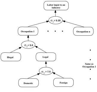
Within industry j’s labor input, the demand for labor by birthplace, legal status and occupation is determined by a nested CES cost minimization problem. The nesting and the substitution elasticities are indicated in Figure 3.2. We assume that there are low substitution possibilities between occupations (substitution elasticity of 0.35) but high substitution possibilities between legal and illegal workers of the same occupation (substitution elasticity of 5) and between domestic and foreign legal workers of the same occupation (substitution elasticity of 7.5). Our choice of 7.5 for the domestic/foreign substitution elasticity is suggested by the econometric work of Ottaviano and Peri (2006). The other substitution elasticities represent judgments. Subsection 6.4 contains relevant sensitivity analysis.
In algebraic terms, we assume that industry j satisfies its labor requirements by choosing:
Figure 3.2. Nesting assumptions in the creation of the labor input to each industry
Labor input to an industry
. . .
.
.
.
.
Same as Occupation 1
Occupation 1 Occupation n
Illegal Legal
Domestic Foreign
= 0.35
= 5.0
= 7.5
σ
1
σ3 σ2
3 t
D (s, o, j) , j’s input of labor of legal status s and U.S. occupation o, defined as a CES aggregate over b of (b,s,o,j) inputs, and
2 t
D (o, j) , j’s input of labor of U.S. occupation o, defined as a CES aggregate over s of (s,o,j) inputs,
to minimize t t
b,s,o
BTW (b,s, o) *D (b,s, o, j)
∑ (3.13)
subject to D ( j)1t =CESo⎡⎣D (o, j)2t ⎤⎦ (3.14)
2 3
t s t
D (o, j)=CES ⎡⎣D (s, o, j)⎤⎦ for all U.S. occupations o, (3.15)
and D (s, o, j)3t =CESb⎡⎣D (b,s, o, j)t ⎤⎦ (3.16)
for all U.S. occupations o and legal status s9.
The CES functions in (3.14) to (3.16) incorporate the elasticities shown in Figure 3.2 and are calibrated to reflect the data on the occupational, birthplace and legal status of workers in U.S. industries.10
9
From problem (3.13) – (3.16) we obtain demand functions of the form
(
)
1
t t b,s,o, j t
D (b, s, o, j)=D ( j) * h BTW (bb, ss, oo) ∀bb, ss and U.S. occupations oo
for all b,s and U.S. occupations and industries o and j. (3.17) These can be aggregated across industries to determine aggregate demand for (b,s) workers in U.S. occupation o as
t t
j
D (b, s, o)= ∑D (b, s, o, j) for all b, s and U.S. occupations o . (3.18)
We assume that employment of (b,s) workers in U.S. occupation o, E (b,s, o) , is t determined by demand:
t t
E (b,s, o)=D (b,s, o) for all b,s and U.S. occupations o . (3.19) 3.5. Relationship between after-tax and before-tax wage rates in the U.S.
As can be seen from the previous sub-sections, after-tax wage rates are important in motivating labor supply while before-tax wage rates motivate demand. To relate after-tax wage rates to before-tax wage rates we include in USAGE-M:
(
)
t t t
ATW (b,s, o)=BTW (b,s, o) * 1 T (b,s)− for all b,s and U.S. occupations o (3.20)
ave
t t t
ATW (b,s, u)=BTW (b,s) * F (b,s) for all b,s and unemployment functions u. (3.21) In these equations,
t
T (b,s) is the payroll and income-tax rate applying to all (b,s) workers in the U.S.;
ave t
BTW (b,s) is the average real before-tax wage rate of (b,s) workers in the U.S.; and
t
F (b,s) is the fraction of BTWtave(b,s) that (b,s) people receive in unemployment activities from social security payments or other support. In the simulations described in sections 4 and 5, we assume that the F (b,s) 'st are unaffected by changes in immigration policies, that is we assume that percentage movements in unemployment benefits match those in average before-tax wage rates.
As can be seen in section 5, in the policy run on the effects of increasing the costs to employers of using foreign-illegal labor, the shock is an increase in T (b,s)t for b = foreign and s = illegal.
3.6. Wage adjustment
In policy runs, we assume that wage rates adjust according to the equation:
t t 1 t t
base base base base
t t 1 t t
ATW (b,s, o) ATW (b,s, o) D (b,s,o) L (b,s,o)
ATW (b,s, o) ATW (b,s,o) D (b,s,o) L (b,s,o)
− −
⎛ ⎞
⎜ ⎟
− = β −
⎜ ⎟
⎝ ⎠
,
for all (b,s) and all U.S. occupations o (3.22)
10
where the superscript “base” refers to values in the basecase forecast and β is a positive parameter.
This equation implies that if a policy causes the market for (b,s,o) employment in year t to be tighter than it was in the basecase forecast (i.e., if the policy causes a larger percentage deviation in demand than supply), then there will be an increase between years t-1 and t in the deviation in (b,s,o)’s real after-tax wage rate. In other words, in periods in which a policy has elevated demand relative to supply, real wages will grow relative to their basecase values. Figure 3.3 illustrates the operation of equation (3.22) for a model with a single employment activity.
Our assumed wage-adjustment process is compatible with a search model [see for example, Bohringer et al. (2005)] in which reductions in labor supply, and resulting reductions in the unemployment rate, generate decreases in the value of having a job relative to the value of not having a job, thereby emboldening workers to demand higher wage rates. It is also compatible with efficiency-wage theory, see for example, Layard et al. (1994, pp. 33-45). Under this theory, employers offer wage rates that optimise worker effort per dollar of wage cost. The theory suggests that the effort-optimising wage rate rises when there is a decrease in labor supply and a consequent temporary decrease in unemployment.
In the context of USAGE-M, we can think of equation (3.22) as having the role of determining after-tax wage rates for occupations in the U.S. Then at given tax rates, equations (3.20) and (3.21) determine before-tax wage rates for these occupations and for unemployment. The only other wage rate in our model is the after-tax wage rate in Mexico. We set this exogenously.
3.7. The determination of everyone’s activity: who gets the jobs and what happens to those who don’t?
Under (3.22), markets for U.S. occupations do not clear. Consequently, we need to specify which offers to employment are accepted and what activities are undertaken by those whose offers to employment are not accepted. In terms of Figure 3.1, we need to specify the downward sloping arrows.
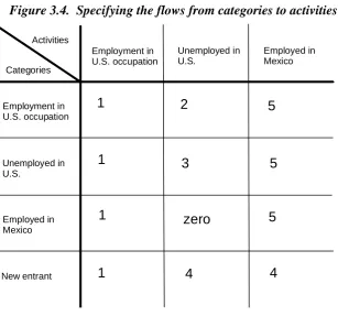
In linking categories at the start of year t to activities in year t, we specify an equation for the flow from each category c to each activity a, Ht(c;a).
Flows from all categories to employment in U.S. occupations(area 1 in Figure 3.4)
We start by defining vacancies in U.S. employment activity a in year t as employment, Et(a), less the number of jobs filled in the activity by people in category a, that is vacancies in a are jobs less those filled by incumbents:
[
]
t t t
V (a)=E (a) H a ; a− for all U.S. employment activities a (3.23)
where
t
V (a) is vacancies and
[ ]
t
Figure 3.3. Wage adjustment in a steady state with one type of employment: a supply shock
α
α
ATW(1)=1 ATW(2) ATW(3)
L(1)=E(1)=1
L(2) L(3) E(3) E(2)
ATW
D
D
S
S
S2
ATW(3) - ATW(2) = α[E(3) - L(3)]
ATW(2) - ATW(1) = α[E(2) - L(2)] ATW( )∞
L( )=E( )=1∞ ∞
S2
In this illustration, but not in USAGE-M, we assume that there is only one type of labor and that the basecase was generated under steady-state assumptions in which technology, consumer tastes, foreign prices, capital availability, taxes, the size of the labor force and other variables affecting the demand for and supply of labor are unchanged from year to year. In this steady state the demand curve for labor (drawn for a given tax rate) is DD and the supply curve is SS. For convenience we assume that the after-tax wage rate, employment and the supply of labor are one in the steady state, allowing us to eliminate the basecase forecasts from equation (3.21). Now consider a policy simulation (e.g. a decrease in migrant inflow) involving a shift in the supply curve in year 2 to S2S2, where it remains for all future years. Assuming that
there is no change in tax rates (so that changes in after-tax wage rates on the vertical axis are also changes in pre-tax wage rates), then employment decreases from E(1) to E(2) to … E(∞), labor supply decreases from L(1) to L(2) and then rises from L(2) to L(3) to … L(∞), and wages rise from ATW(1) to ATW(2) to … ATW(∞).
The flow of people from category c to U.S. employment activity a, a ≠ c, is modelled as being proportional to the vacancies in a and to the share of category c in the supply of labor to activity a from people outside category a. Thus, if people in category c account for 10 per cent of the people outside category a who want jobs in employment-activity a, then people in category c fill 10 per cent of the vacancies in a. That is,
t
t t
t s a
L (c; a) H (c ; a) V (a) *
L (s; a)
≠
∑
⎡ ⎤
⎢ ⎥
= ⎢ ⎥
⎢ ⎥
⎣ ⎦
,
Figure 3.4. Specifying the flows from categories to activities
Activities
Categories
Employment in U.S. occupation
Unemployed in U.S.
Employed in Mexico
Employment in U.S. occupation
Unemployed in U.S.
Employed in Mexico
New entrant
1
1
1
1
2
3
zero
4 4
5
5
5
In (3.24), we assume that there is always competition for jobs, that is we assume that the number of people from outside category a who plan to work in employment-activity a,
s a≠ L (s; a)t
∑ , is greater or equal to the number of vacancies [V (a) ] in a.t 11 This ensures that H (c;a)t is less than or equal to L (c;a)t for all categories c ≠ a and all U.S. employment activities a.
A familiar idea in labor economics is that unemployed people, especially long-term unemployed people, have a lower probability of filling vacancies than employed people wanting to move. This idea could be handled in (3.24) by attaching weights to the L's appearing on the RHS. We achieve a similar effect by assuming that the unemployed, especially the long-term unemployed, make comparatively weak offers to employment. [Recall the last two dot points in our discussion of the Bt(c;a)’s.] That is,
U.S. emloy activ t t a∈ L (c; a) / CAT (c)
∑ is low for people in unemployment categories c.
The number of incumbents in employment-category c who remain in activity c
t
[H (c;c)] is defined as the number of people in category c less the number who move out of activity c:
t t t
a c
H (c; c) CAT (c) H (c; a)
≠
∑
= − , for all employment categories c (including Mexico) (3.25) With [H (c; a)] being less than or equal to t [L (c; a)] for a t ≠ c, H (c; c) is greater than or t equal to L (c;c)t . People in employment-category c who planned to work in activity a ≠ c but who are unable to move to a due to insufficient vacancies simply remain in c.
11
Flows from all U.S. employment categories to U.S. unemployment activities (area 2 in Figure 3.4)
People in a U.S. employment category at the start of year t cannot move to a long-run unemployment activity. If they move into unemployment it must be to short-long-run unemployment. The number of people who make the move to short-run unemployment is the sum of two parts: voluntary moves, Lt(c;u), and involuntary moves. We model involuntary moves from U.S. employment category c as a fraction, μ(c), of the number of people in the category:
for short run unemployment activities u
for long run unemployment activities u
c t
t
L (c; u) (c) * CAT (c)
H (c; u) 0 − − + μ ⎧ = ⎨ ⎩
for all U.S. employment categories c , (3.26) Normally, μ(c) is exogenous. However, it is possible that (3.26) in conjunction with (3.24) will give values for Ht(c;c) in (3.25) that exceed Et(c). In this case, Vt(c) would be negative. We avoid this situation by treating μ(c) as an endogenous variable. If Vt(c) is greater than zero, then μ(c) equals an exogenously given minimum value determined by the rate at which individuals are dismissed because of their performance or other factors unrelated to overall demand for people in activity c. Alternatively, μ(c) moves sufficiently above its minimal value to ensure that Vt(c) equals zero. When μ(c) is above its minimum value, then there are involuntary flows from employment category c to unemployment caused by overall shortage of jobs.
Flows from U.S. unemployment categories to U.S. unemployment activities (area 3 in Figure 3.4)
Next we deal with flows between unemployment categories and unemployment activities. We ensure that short-term unemployed people who fail to obtain a job flow to long-term unemployment; and that long-term unemployed people who fail to obtain a job remain in long-term unemployment:
for short run unemployment activities u
for long run unemployment activities u a employment activ
t
t t
0
H (c; u) CAT (c) H (c; a)
− − ∈ ∑ ⎧⎪ = ⎨ − ⎪⎩
for all U.S. unemployment categories c and all unemployment activities u . (3.27)
Flows from New categories to U.S. unemployment activities or to Mexico (area 4 in Figure 3.4)
New legal entrants (either domestic or foreign) who fail to get a U.S. job are allocated to a short-run unemployment activity. New illegal entrants who fail to get a U.S. job are allocated to employment in Mexico. These allocations are specified by:
for c not foreign, illegal and for short run unemploy activ u a U.S. employ activ
for c foreign, illegal and for Mexican activities u a U.S. employ activ
otherwise
t t
t t t
CAT (c) H (c; a)
H (c; u) CAT (c) H (c; a)
0 − ∈ ∈ ∑ ∑ − ⎧ ⎪ ⎪ =⎨ − ⎪ ⎪⎩
Flows from non-New categories to Mexico (area 5 in Figure 3.4)
We assume that flows to Mexico from non-Mexican, non-New categories are voluntary. This means that foreign illegal workers in the U.S. can go home if they want to. Finally, the flow from the category of working in Mexico to the activity of working in Mexico is determined as the number of people in the category less the number that obtain jobs in the U.S. Thus we have:
for c non Mexican
for c Mexican a U.S. employ activ
t t
t t
L (c; u)
H (c; u) CAT (c) H (c; a)
−
∈ ∑
⎧⎪
= ⎨ −
⎪⎩
for all non-New categories c and for Mexican activities u (3.29)
Completing the link from categories to activities
To complete the link from categories at the start of year t to activities in year t we include the equation:
t t
c
H (c, a) E (a)
∑ = , for all U.S. unemployment activities and Mexican activities a
(3.30)
A similar equation is not required for U.S. employment activities. Such an equation is implied by (3.23) and (3.24).
4. Restricting the supply of foreign-illegal labor to the U.S.
In this section we use USAGE-M to compute the effects on the U.S. economy of a policy of tighter border security that raises the costs to illegal migrants of entering the U.S. The policy shock is introduced as a 25 per cent reduction in the marginal utility to potential illegal migrants from earning money in the U.S. We refer to the simulation as simulation SR (Supply Restriction).
From the point of view of supply decisions by potential illegal migrants, the policy shock is equivalent to a 25 per cent reduction in the wage that they anticipate receiving in the U.S. if they make a successful entry. Another way to think about the policy shock is as an increase in the difficulties faced by smugglers in organizing illegal border crossings.12 This could be expected to increase smugglers’ fees. These fees currently average about $4,000 per illegal migrant. For a potential illegal migrant who plans to stay in the U.S. for one year and who anticipates earning $20,000, the policy shock is equivalent to an increase smugglers’ fees to about $9,000 (an increase of $5,000 or 25% of $20,000).
In terms of equation (3.8) in section 3, the shocks in the policy run are a 25 per cent reduction in Bt(c;a) for c = (foreign, illegal, Mexico or New) and a = (foreign, illegal, o) where o is any U.S. occupation. The shocks are introduced as 13.4 per cent reductions in both 2006 and 2007.
4.1. Net and gross flows of illegal migrants into U.S. employment
Chart 4.1 shows the employment paths for illegal migrants in the basecase and the policy runs. In the basecase (without the policy shocks), employment of illegal migrants grows between 2005 and 2019 at 3.8 per cent a year, from 7.3 million to 12.4 million. By contrast, the employment of legal residents through this period grows by only 1.0 per cent a year. The share of illegal migrants in total employment increases from 4.98 per cent in 2005 to 7.17 per cent in 2019. Because illegal migrants have low-paid jobs, their share in the total wagebill is considerably less than their share in total employment. In our basecase, their wagebill share goes from 2.69 per cent in 2005 to 3.64 per cent in 2019.
12
In creating the basecase, we recognised that population growth in Mexico is slowing and that, in the absence of fresh U.S. policy initiatives, growth in net inflow of illegal migrants is likely to be quite moderate over the next 15 years.13 We assume average annual growth of net inflow of illegal migrants to U.S. employment of one per cent. Nevertheless, the number of illegal migrants in the U.S. will grow rapidly. This is because the current net inflow to U.S. employment (about 400,000) is high relative to the stock of illegal migrants in U.S. employment (7.3 million). Thus, even with only slow growth (1%) in net inflow, or even no growth, strong growth in foreign-illegal employment is assured.
In the policy run, foreign illegal employment grows between 2005 and 2019 at 1.4 per cent a year, from 7.3 million to 8.9 million. Thus the policy has the effect of reducing foreign-illegal employment in 2019 by 3.55 million (=12.4 – 8.9) or 28.6 per cent.
Chart 4.2 shows that the policy of tighter border security affects flows of illegal migrants in both directions. The shocks have a direct effect on inflows by reducing the number of people in Mexico who want to move illegally to the U.S. Via (3.8) there is a reduction in Lt(c;a) for c = (foreign, illegal, Mexico or New) and a = (foreign, illegal, o) where o is any U.S. occupation. The shocks have an indirect effect on outflows by lowering the number of illegal migrants present in the U.S. and thereby lowering the number who seek to go home. In terms of our model, the shocks reduce the number of people in those categories in the U.S. that offer to supply labor to Mexico, that is, the shocks reduce the number of people in CATt(c) where c is a foreign-illegal category in the U.S.
There are two features of Chart 4.2 that require further comment. First, it implies that the net inflow to the U.S. workforce of foreign illegals of about 400,000 in 2005 was generated by a gross inflow of about 1 million and a gross outflow of about 600,000. These numbers are consistent with foreign illegal migrants making frequent trips home. However, there are no firm data on gross flows. Fortunately we have found that our results for the effects of reducing foreign-illegal employment in the U.S. are not sensitive to our assumptions concerning the initial levels of gross flows.
The second notable feature of Chart 4.2 is the sharp decline in the early years of the policy run in the net and gross inflows of foreign illegals to U.S. employment, followed by recovery in later years. It appears that increased border security would have a much greater effect on flows of illegal migrants in the short run than in the long run.
To explain this result we start with (3.8). This equation suggests that the initial impact of the policy shocks is a 44% decline in supply from Mexico.14 However, the policy-induced decline in gross inflow shown in Chart 4.2 for 2007 is 84 per cent and the net inflow in the policy run is negative. The impact decline (44 per cent) in supply from Mexico causes an increase in foreign-illegal wages (equation 3.21) and a decrease in U.S. demand for illegal labor (equation 3.16): the growth rate in demand for foreign-illegal labor for the period 2005 to 2007 turns from strongly positive in the basecase to
13
This view is partially supported by Hanson and McIntosh (2007) who emphasise the link between Mexican population growth and net inflow of migrants to the U.S. Against this, they also point out that network effects are important. The current large Mexican population in the U.S. will encourage further inflow by providing a support network in the U.S. for potential new migrants.
14