Analyzing the dynamic structure of liquid metals and alloys
Jean-FrançoisWax1,∗and TarasBryk2,3
1Laboratoire de Chimie et de Physique-A2MC, Université de Lorraine-Metz, 1, boulevard Arago 57078
Metz Cedex 3, France
2Institute for Condensed Matter Physics, National Academy of Sciences of Ukraine, 1 Svientsitskii
Street, UA-79011 Lviv, Ukraine
3Institute of Applied Mathematics and Fundamental Sciences, Lviv Polytechnic National University,
UA-79013 Lviv, Ukraine
Abstract.Experimental and numerical improvements have stimulated a great interest in the dynamic structure of liquids during the last decades. Many unex-pected features have been unveiled among which fast sound, positive dispersion and possible coupling between transverse and longitudinal excitations can be mentioned. Models used to analyze these data have to be sound and more and more rigorous. In this study, we discuss the capability of a recently proposed fitting scheme (Wax J.-F. and Bryk T. J. Phys.: Condens. Matter25325104 (2013); 26 168002 (2014). Wax J.-F., Johnson M.R., and Bryk T. J. Phys.: Condens. Matter28185102 (2016).) to interpret these features of the dynamic structure of liquid metals and alloys.
1 Introduction
Experimental techniques used to measure the dynamic structure of liquids, namely neutron or x-ray inelastic scattering, have made great progress during these last two decades. This allows to investigate dynamic properties with unprecedented accuracy. This is also true for simulation techniques which have benefited from the constant increase in available comput-ing power. While the description of the interactions seems not to be a problem anymore as dynamic structure can now be obtained from ab-initio methods with a correct statistical ac-curacy, we are faced with a new challenge. Indeed, analyzing experimental or simulation results requires now accurate models in order to correctly interpret the observed features and not to be deluded with fitting artifacts. It is also important that parameters involved in the models have a concrete meaning in order to trace each contribution to the structure back to their origin.
In this work, a recently developed analysis scheme [1–3] inspired from the Generalized Collective Modes (GCM) approach [4] is presented and applied to simulation results of liquid metals and alloys. We focus on three features revealed by increasing accuracy of available data, namely the positive dispersion of acoustic waves in pure liquids, the so-called "fast sound" effect in mixtures and finally the possible coupling between transverse and longitudi-nal excitations. Beyond presenting this alongitudi-nalysis scheme, its advantages and limitations, the purpose of this work is also to point out some aspects at which attention should be paid when fitting data.
After this introduction, important notions about dynamic structure will be recalled, namely how is it described and determined, as well as the concept of collective modes lead-ing to the model that we proposed. In the third section, this model will be applied to the analysis of three topics: positive dispersion, fast sound and coupling between longitudinal and transverse excitations. Finally, we will summarize the main conclusions of this work.
2 Dynamic structure
2.1 Description and determination
In order to describe the dynamic structure of a liquid, several functions can be introduced that are all derived from the van Hove functionG(r,t). The intermediate scattering function
F(q,t)=
G(r,t) exp (iq.r)dr= 1 N
N
a=1
e[iq.ra(0)].N b=1
e[−iq.rb(t)]
(1)
is its space Fourier transform; it can be computed directly from the positions obtained from molecular dynamics (MD) simulations. The dynamic structure factor
S(q, ω)= 1 2π
+∞
−∞ F(q,t) exp(iωt)dt (2)
is the time Fourier transform ofF(q,t); it is also obtained directly from inelastic scattering experiments (of x-rays or neutrons). Finally, the current correlation functionJ(q, ω) can be deduced fromS(q, ω) by simply multiplying it byω2/q2.
In the case of an alloy of two species 1 and 2, we need to consider the chemical nature of the atoms. Therefore, partial functions are introduced. For a binary mixture, three partial structure factors are needed to obtain a complete description. This is also the case for the other functions. Partial functions can easily be obtained from simulation, but experiments usually only provide with a single total weighted function which, in the case of neutrons, reads
FINS(q,t)=
c1b21F11(q,t)+2√c1c2b1b2F12(q,t)+c2b22F22(q,t) c1b21+c2b22
(3)
which is a linear combination of the partial ones, wherebiare neutron scattering amplitudes of corresponding atoms. The difficulty is then to disentangle the three contributions. It should also be recalled that partial functions of the Bhatia and Thornton’s kinds can also be used. They describe the system in terms of atom number and concentration.
These functions have mathematical properties called sum-rules. +∞
−∞ S(q, ω)dω = F(q,0)=S(q), (4) +∞
−∞ ωS(q, ω)dω = i
∂F(q,t) ∂t
t=0=0, (5)
+∞
−∞ ω
2S(q, ω)dω = −∂2F(q,t)
∂t2
t=0=q2kBT/m, (6) +∞
−∞ ω
3S(q, ω)dω = −i ∂3F(q,t)
∂t3
t=0=0 (7)
J(q, ω) must tend to zero asωtends to infinity. Models used to interpret the data should obey as many of these sum rules as possible. Of course, similar relations also exist in the case of alloys.
In order to determine these functions, on the experimental side, dynamic structure can be probed at the atomic scale by inelastic neutron or x-rays scattering. This last technique has benefited from the advent of high flux synchrotron sources which has strongly boosted the study of dynamic structure over the last two decades. The function that is obtained is the dynamic structure factorS(q, ω). On the simulation side, usual limitations are of course recovered in terms of accuracy of the interactions for classical MD, and of statistical accuracy for ab-initio simulations. However, the results do not need to be corrected from experimental side-effects. Moreover, partial functions are easily computed in the case of alloys, as well as transverse dynamics ones. The function usually computed is the intermediate scattering functionF(q,t).
2.2 Collective modes
A central concept used to analyze the dynamic structure of a liquid is that of collective modes. It can be understood looking at the shape of the dynamic structure factor that is usually composed of several peaks. Each peak corresponds to one or more modes, so that the dynamic structure stems from sum of contributions from several modes. They can be of relaxing or of propagating kind and can easily be distinguished. Propagating modes usually contribute to side peaks inS(q, ω) while relaxing modes contribute to the central peak. Looking atF(q,t), the propagating ones appear as oscillations while the relaxing ones contribute as exponential decays [3].
There is one (ω,q) domain in which the leading contributions to S(q, ω) are well-understood: the macroscopic limit which corresponds to the hydrodynamic model. In this length and time ranges, conservation rules of particle density, momentum and energy lead to slow long-lived collective modes which give rise to well-defined sharp peaks. The central one, called Rayleigh peak, is connected to thermal relaxations, because macroscopic adia-batic propagation of sound causes small differences in local temperature for compressed and uncompressed regions. The pair of side peaks, called Brillouin peaks, correspond to density waves related to sound propagation. The side-peak positions are connected with the sound velocity and the dispersion curve is linear in this range. In the case of alloys, another quantity is conserved, namely the chemical composition which leads to a second contribution to the central peak from relaxation connected with mutual diffusivity of species.
At interatomic distances, we enter the so-called kinetic regime and additional modes con-tribute to the dynamic structure measured in x-rays or neutrons experiments. Kinetic modes include structural relaxation and thermal waves, for instance. It is very easy to distinguish between hydrodynamic and kinetic modes. In order to propagate over macroscopic distances, the damping of hydrodynamic modes must tend to zero withq. Conversely, kinetic mode be-come evanescent on long distances and their damping tend to a non-zero value in the same limit. It is also useful to notice that, at a givenq-value, two coupled relaxation modes with comparable relaxation times can mix into a propagation mode and vice-versa.
2.3 Model used
consistent picture as to the origin of the various modes involved. This approach adds kinetic modes to the hydrodynamic description by taking into account non-hydrodynamic variables. By determining the eigen-functions and eigen-values of the collective variables obtained from MD simulations, it can determine the collective modes and their contributions to the dynamic structure functions. We shall call "full-GCM" this method which allows to understand quite completely the nature of the mechanisms involved in the dynamic structure. Of course, it cannot be applied directly to experimental data. But, interestingly, it leads to expressions that are rather simple and that we can easily use to fit experimental or simulation results.
Therefore, we consider the following expression:
F(q,t)= Nr
i=1
Aiexp [−αi.t]+ Np
j=1 Bjexp
−βj.t
cosωj.t+ϕj
. (8)
Relaxing modes are depicted by exponential decays, while propagating modes are taken into account by damped cosine functions. S(q, ω) and J(q, ω) also have analytic expressions. Fitting parametersAi,αi,Bj,βj,ωj, andϕjareqdependent quantities. The number of modes depends on the system considered, but anyway, we are faced with the question of the number of free parameters. Indeed, considering just one relaxing mode and one propagating mode would lead to six independent parameters in a pure liquid.
In order to reduce this number, we found it useful to consider the sum-rules mentioned before. For instance, introducing the first three relations, we were able to reduce the number of independent parameters down to three in the case of two modes for pure liquids [1]. But the most important is that this guarantees a correct asymptotic behavior of dynamic structure functions and especially of J(q, ω) (see Ref. [2] for a comparison with Damped Harmonic Oscillator (DHO) model which leads to a wrong high frequency asymptote ofJ(q, ω) when combined with a central lorentzian due to wrong behavior of this latter). This model appeared to be efficient whatever theq-value (before, after, or at the position of the first peak ofS(q)), in the case of both pure liquids and alloys.
3 Results and discussion
We turn now to some topics of interest that can be highlighted using our model. We will discuss first the so-called positive dispersion, then the fast sound, and finally, the possible coupling between transverse and longitudinal modes. These topics show increasing com-plexity.
3.1 Positive dispersion
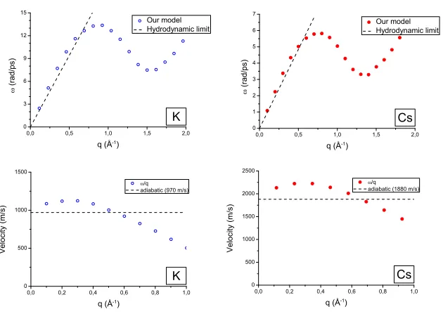
Figure 1.Dispersion curves (first line) and apparent speed of soundω/q(second line) for liquid K and Cs. Asymptotic hydrodynamic limit is also drawn.
In Figure 1, we have plotted the dispersion curves corresponding to our studies of K [2] and Cs [3]. These results were obtained from simulations with 2048 particles in a thermody-namic state close to the melting point. The results were analyzed using our model involving one relaxation mode and one propagation mode and three sum-rules were fulfilled. Complete details about the procedure can be found in Refs. [1, 2]. The hydrodynamic asymptote is also plotted. In order to illustrate quantitatively the positive dispersion, it is convenient to con-sider the quantityω/qwhich dimension is velocity. In these curves, the positive dispersion is clearly visible and reaches 18 % for potassium and 16 % for cesium.
As a conclusion about this point, it should pointed out that: (i) the phenomenon is clearly visible and confirmed by our model; (ii) the parameters obtained smoothly vary withq. Try-ing to add additional modes leads to scattered data for this mode; (iii) a fit remains a fit and we can not determine the origin of the phenomenon from it alone. A deeper analysis is required. For instance, using full-GCM approach [6], it has been possible to connect the existence of positive dispersion to a coupling between sound excitation and non-hydrodynamic structural relaxation. The hypothesis of a coupling of sound propagation with hydrodynamic thermal relaxation (leading to negative dispersion) has been ruled out by this study.
3.2 Fast sound
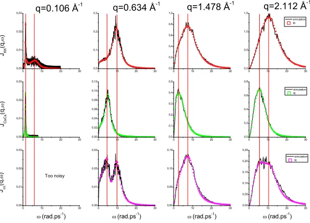
Figure 2. PartialJ(q, w) functions, namely K-K, Cs-Cs, and Bhatia-ThorntonC−Cfor K-Cs alloy. Solid lines are raw simulation data while open squares are the curves fitted using our model. The vertical red lines are only guide for the eyes corresponding to positions of the maximum.
As the second branch appears to have a slope higher than the branch corresponding to the adiabatic speed of sound, this phenomenon has been called "fast sound". However, only one such branch survives in the hydrodynamic limit and a lively debate followed about the exact nature and origin of this phenomenon. For instance, it was believed for a long time that it could only exist in mixtures with high mass-ratio between its components.
It could never have been understood without simulation. Indeed, the answer lies in the partial structure functions which are out of reach of experiment. On a technical point of view, it is also necessary to define a correct fitting function, taking care to the fact that the number of independent parameters remains reasonable in order to remain meaningful.
Results for liquid K-Cs alloy at equiatomic composition [3] are presented in Figure 2. The partial dynamic structure functions were fitted considering two relaxation and two prop-agation modes. The first two sum-rules were applied. In this alloy, the mass-ratio is about 3.4 and only one dispersion branch had been observed experimentally [10].
Looking at the parameters of these modes (not shown here, please refer to [3]), consid-ering first their frequencies, the low frequency is very similar to the corresponding pure Cs branch. On the other hand, the high frequency branch has only remote resemblance with the pure potassium branch and, notably, it tends to a non-zero limit asqtends to zero. Looking at the damping, this mostly indicates that the low-frequency mode is of hydrodynamic nature, while the high-frequency one is kinetic. Of course, what we have been able to highlight in the case of K-Cs with a rather low mass-ratio can also be observed in the case of mixtures with high ratio like Li-Tl or Li-Bi, for instance.
To conclude this part, two aspects should be mentioned. The first one is the importance of considering the partial functions and theirq-dependent contributions to the total correlation functions, and thus, the strategic position of numerical simulation. The second one, is that fitting such an intricate wealth of data requires a well established model which should be as rigorous as possible. Otherwise, the same data set could lead to very different sets of results.
3.3 Longitudinal/Transverse coupling
Transverse excitations should not be observed in the first Brillouin zone in inelastic scatter-ing experiments. However, a discussion has been opened a few years ago when Hosokawa and co-workers [11] claimed anomalies in their measurements of Ga. This anomaly for wave numbers inside the first pseudo-Brillouin zone has also been reported in Na [12], Sn [13], Cu, Fe [14], and Zn [15]. On the basis of a DHO fit, they noticed the coincidence between the anomaly and the transverse excitations frequencies obtained by simulation. Thus, it was proposed that these anomalies could be attributed to transverse modes. But up to now, no the-oretical model predicts the existence of such transverse mode contribution. Moreover, MD simulations performed for several liquid metals do not show evidences of identical peak fre-quencies in longitudinal and transverse current correlation functions when the wave numbers are within the first pseudo-Brillouin zone [16, 17].
As fit is sensitive to the model used, we search for another possible explanation [17]. In order to discuss the possible origins of the anomaly detected in the data of several metals, we performed ab-initio simulation of sodium. To analyze the data, we considered several methods. We computed the longitudinal structure functions and fitted the data using two propagating modes. We first analyzed these modes using two DHO functions fulfilling one sum-rule, then using two GCM functions (see Eq.8) fulfilling three sum-rules. We also com-puted the transverse waves that propagate in the kinetic range and performed a full-GCM analysis of the data.
The results are plotted in Figure 3. The acoustic branch obtained from peak positions of J(q, ω) agrees favorably with experimental data. Additional modes obtained considering two DHO’s and two GCM contributions are different, illustrating the relevance of fulfilling as many sum-rules as possible. This also demonstrates that both approaches confirm the existence of a minor second mode. If we now consider the transverse excitations, they are located between both fits. This proximity is the main argument in favor of the coupling between longitudinal and transverse modes. But, if we consider full-GCM results, this theory predicts that thermal waves propagate at about the same frequencies as those by the two GCM fit at wave-vectors lower than the first peak position. The advantage of this explanation is that it is consistent with existing theoretical model. Of course, in the first peak region, the huge structural relaxation contribution prevents to get accurate data about the minor second mode by fitting procedures.
Figure 3. Frequencies of the collective excitations. Experimental and computed acoustic waves are plotted as dotted lines and open red squares, respectively. Additional modes frequencies obtained using two DHO and two GCM functions are plotted as full circles and full squares, respectively. Transverse mode and heat waves frequencies are drawn as solid and dashed lines, respectively.
complexities). Indeed, between two DHO’s and two GCM, important differences appear. Finally, instead of coupling with transverse excitations, we propose another explanation about the nature of this propagating mode that could be heat waves.
4 Conclusion
Considering three different phenomena observed in the dynamic structure of liquid metals and alloys, we have illustrated the capability of a recently proposed fitting model derived from GCM approach. This model can be applied to either simulation or experimental results. The parameters of the collective modes contributing to the functions obtained can be understood in the light of full-GCM results.
However, the following point should be remembered: a fit remains a fit and the results obtained depend on what one put in the model. Tracking additional modes, for instance, leads to additional parameters and very scattered results if the modes are weakly contributing to the data. Available safety barriers like sum-rules or considering simultaneously several functions (F, S, and J) should not be neglected. As the overall accuracy of both experimental and simulation determinations of the dynamic structure keeps increasing, we hope that this model will help improving our understanding of the dynamic structure of liquids and alloys.
References
[1] Wax J.-F. and Bryk T., J. Phys.: Condens. Matter25, 325104 (2013);26168002 (2014). [2] Wax J.-F. and Bryk T., AIP Conf. Proc.1673, 020010 (2015).
[3] Wax J.-F., Johnson M.R., and Bryk T., J. Phys.: Condens. Matter28, 185102 (2016). [4] Bryk T. and Chushak Y., J. Phys.: Condens. Matter9, 3329 (1997).
[5] Scopigno T., Ruocco G., and Sette F., Rev. Mod. Phys.77, 881 (2005).
[6] Bryk T., Mryglod I., Scopigno T., Ruocco G., Gorelli F., and Santoro M., J. Chem. Phys. 133, 024502 (2010).
[7] Jacucci G., Ronchetti M., and Schirmacher W., J. Phys. (Paris) Coll.C8, 385 (1984). [8] Bosse J., Jacucci G., Ronchetti M., and Schirmacher W., Phys. Rev. Letters57, 3277
(1986).
[9] Montfrooij W., Westerhuijs P., de Haan V.O., and de Schepper I.M., Phys. Rev. Letters 63, 544 (1989).
[10] Bove L.E., Sacchetti F., Petrillo C., and Dorner B., Phys. Rev. Letters85, 5352 (2000). [11] Hosokawa S., Inui M., Kajihara Y., Matsuda K., Ichitsubo T., Pilgrim W.-C., Sinn H., González L.E., González D.J., Tsutsui S., and Baron A.Q.R., Phys. Rev. Letters 102, 105502 (2009).
[12] Giordano V.M. and Monaco G., Proc. Natl. Acad. Sci. U.S.A.107, 21985 (2010). [13] Hosokawa S., Munejiri S., Inui M., Kajihara Y., Pilgrim W.-C., Ohmasa Y., Tsutsui S.,
Baron A.Q.R., Shimojo F., Hoshino K., J.Phys.: Condens. Matter25, 112101 (2013). [14] Hosokawa S., Inui M., Kajihara Y., Tsutsui S., Baron A.Q.R., J.Phys.: Condens. Matter
27, 194104 (2015).
[15] Zanatta M., Sacchetti F., Guarini E., Orecchini A., Paciaroni A., Sani L., and Petrillo C., Phys. Rev. Letters114, 187801 (2015).
[16] Bryk T., Ruocco G., Scopigno T., and Seitsonen A.P., J. Chem. Phys., 143, 110204 (2015).