Enhanced Query Optimization Using R Tree
Variants in a Map Reduce Framework for
Storing Spatial Data
Vaishnavi S 1, Subhashini K 2, Sangeetha K 3, Nalayini C.M 4
1,2,3
B.Tech Information Technology, Velammal Engineering College,Chennai, TamilNadu, India.
4
Velammal Engineering College,Chennai, TamilNadu, India.
ABSRACT: The Map-reduce has become one of the inevitable programming framework for developing distributed data storage and information retrieval (IR) [1].Efficient method for mining data and its fast retrieval has become the key concern over years. Various indexing mechanisms have been developed in Hadoop Map-reduce framework, an open-source implementation of Google. The framework consist of two basic functions- the map() function which partition the input into smaller sub-problems and distribute them to worker nodes, the reduce() function which aggregate the sub-outputs from the worker nodes to retrieve the final output. Map-reduce possess certain benefits compared to traditional file system viz locality optimization, very large computation and so on. Hadoop Distributed File System(HDFS) use B+ tree and various other indexing mechanisms where the storage and optimized retrieval of spatial data is an issue[2]. This paper provide an intuitive approach to incorporate Hilbert R tree and priority R tree, variants of R tree, for performing efficient indexing in a map-reduce framework. Priority tree can be considered as a hybrid between K-dimensional tree and R tree that define a given objects N-dimensional bounding volume as a point in N-dimensions, represented by ordered pair of rectangles enhancing quick Indexation [3]. Hilbert R tree, on other hand, can be thought as an extension to B+ tree for multi-dimensional object in spatial database achieving high degree of space utilization and good response time. This is done by proposing an ordering on R tree nodes by sorting rectangles according to Hilbert value of the center of rectangles. Given the ordering, every node has a well-defined set of sibling nodes. Thus, deferred splitting can be used. By adjusting the split policy, the Hilbert R tree can achieve high utilization as desired.
KEYWORDS-Map-reduce framework, Priority R-tree, K-dimensional tree, Hilbert R-tree, Hilbert value, Spatial database.
I) INTRODUCTION
The map reduce is a widely used data parallel program modeling for large scale data analysis. The framework is shown to be scalable to thousands of computing nodes and reliable on commodity clusters. Map-reduce possess certain benefits compared to traditional file system viz ease of use for novice database user, fault tolerance, locality optimization and load balancing, very large computation and dynamic scaling. In particular, Hadoop, an open source implementation of map reduce has become more and more popular in organization, business companies and institutes. Programs in Hadoop map reduce are expressed as map and reduce operations. The map phase takes in a list of key-value pairs and applies the programmer’s specified map function independently on each pair in the list. The reduce phase operates on a list, indexed by a key, of all corresponding values and applies the reduce function on the values; and outputs a list of key-value pairs. Each phase involves distributed execution of tasks(application of the user-defined functions on a part of the data). The reduce phase must wait for all the map tasks to complete, since it requires all the values corresponding
to each key. In order to reduce the network overhead, a combiner is often used to aggregate over keys from map tasks executing on the same node [4].
There are various clustering techniques employed in map reduce environment namely K-means [7] which is
the most basic and simplest unsupervised learning algorithms that solve the well-known clustering problem. The procedure follows a simple and easy way to classify a given data set to a certain number of clusters. On the other hand, the canopy clustering algorithm is an unsupervised pre-clustering algorithm, often used as pre-processing step for the K-means algorithm or the hierarchical clustering algorithm. It is intended to speed up clustering operations on large data sets, where using another algorithm directly may be impractical due to the size of the data set. The algorithm proceeds as follows:
Cheaply partitioning the data into over lapping subset(called “canopies”)
Perform more expensive clustering, but only within this canopies.
Complexity analysis is another technique where most of the work is done by the mapper and the work load is pretty balanced. So the time complexity will be O(k*n/p) where k is number of cluster, n is number of data points and p is number of machines.
The clustering technique is accompanied with various indexing techniques that can be implemented using balanced trees, B+ trees and Hashes. Map reduce predominantly uses B, B+ tree for implementing indexation. A balanced tree is a binary search tree that automatically keeps its height(number of levels below the root) small in the face of arbitrary item insertions and deletions. The B tree is the classic disk-based data structure for indexing records based on an ordered key set. The B+ tree is a variant of the original B tree in which all records are stored in the leaves and all leaves are linked sequentially. The B+ tree is used as an indexing method in relational database management system. A Hash table or Hash map is a data structure that uses a hash function to map identifying values, known as keys, to the associated values. Thus, a hash table implements an associative array. The hash function is used to transform the key into the index of an array element where the corresponding value is to be sought.
II) THE EXISTING INDEXATION IN MAP-REDUCE
primary storage (RAM). Instead, a relatively small portion of the data structure is maintained in primary storage, and additional data is read from secondary storage as needed. Unfortunately, a magnetic disk, the most common form of secondary storage, is significantly slower than random access memory (RAM). In fact, the system often spends more time retrieving data than actually processing data. Effective optimization in map reduce is achieved through various indexing algorithms and implementing trees for efficient sorting of data. The traditional method of implementation is B and B+ tree that are the descendent of binary tree. The B-tree is a generalization of a binary search tree in that a node can have more than two children. The B-tree is optimized for systems that read and write large blocks of data. For n greater than or
equal to one, the height of an n-key b-tree T of
height h with a minimum degree t greater than or equal
to 2,
In a B+ tree, in contrast to a B-tree, all records are stored at the leaf level of the tree; only keys are stored in interior nodes. The leaves (the bottom-most index blocks) of the B+ tree are often linked to one another in a linked list; this makes range queries or an (ordered) iteration through the blocks simpler and more efficient (though the aforementioned upper bound can be achieved even without this addition). This does not substantially increase space consumption or maintenance on the tree. This illustrates one of the significant advantages of a B+ tree over a tree; in a B-tree, since not all keys are present in the leaves, such an ordered linked list cannot be constructed. A B+ tree is thus particularly useful as a database system index, where the data typically resides on disk, as it allows the B+-tree to actually provide an efficient structure for housing the data itself [5].
However, the real-time data may also involve three-dimensional objects like lines, polygons and so on. Storage of spatial data is of great concern. To counter the issue, map reduce started to develop R tree for efficient indexation and storage of spatial data [6]. In
this regard, the base knowledge of spatial data is considered to be of importance.
A. Spatial Database –An Overview
A Spatial database is a database that is optimized to store and query data that is related to objects in space, including points, lines and polygons [2]. While typical
databases can understand various numeric and character types of data, additional functionality needs to be added for databases to process spatial data types. Database systems use indexes to quickly look up values and the way that most databases index data is not optimal for spatial queries. Instead, spatial databases use a spatial index to speed up database operations. Spatial indexes are used by spatial database to optimize spatial queries. Indexes used by non-spatial databases cannot effectively handle features such as how far two points differ and whether points fall within a spatial area of interest. Common spatial index methods includes R tree
(Typically the preferred method for indexing spatial data. Objects are grouped using the minimum bounding rectangle (MBR). Objects are added to an MBR within the index that will lead to the smallest increase in its size.), R+ tree (a variant of R tree for spatial data), R* tree(R*-trees support point and spatial data at the same time with a slightly higher cost than other R-trees)
B. Performance of B+ Tree and R Tree
The relative performance of B+ tree depends on characteristics like work load composition, the system resource available, the B+ tree structure and multi-programming level. The R tree retrieve the spatial data in an efficient manner while B tree and its variants are employed only for linear database. The performance of R tree in terms of space utilization, communication cost and resource usage is found to be two to three times more than that of B+ tree [5]. Further specification in
terms of graphs and comparison chart has been presented in the following sections.
III) THE PROPOSED OPTIMIZATION USING HILBERT AND PRIORITY R TREE
In order to handle spatial data efficiently, as required in computer aided design and geo-data applications, a database system needs an index mechanism that will help it retrieve data item quickly according to the spatial locations. However, traditional indexing methods are not well suited to data objects of non-zero size located in multi-dimensional spaces. An index based on object spatial locations is desirable, but classical one-dimensional database indexing structures are not appropriate to multi-dimensional spatial searching. Structures based on exact matching of values, such as hash tables, are not useful because a range search is required. Structures using one-dimensional ordering of key values, such as B tree and its variants, do not work because the search space is multi-dimensional. A Spatial database consist of a collection of tuples representing spatial objects, and each tuple has a unique identifier which can be used to retrieve it. Hence we propose to in-corporate Hilbert R tree and Priority R tree to handle multi-dimensional data.
A. Hilbert R Tree and its Operation
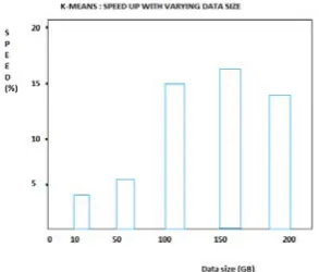
Figure 1: K means variation with data size
The dynamic Hilbert R-trees employ flexible deferred splitting mechanism to increase the space utilization. Every node has a well defined set of sibling nodes. By adjusting the split policy the Hilbert R-tree can achieve a degree of space utilization as high as is desired. This is done by proposing an ordering on the R-tree nodes. The Hilbert R-tree sorts rectangles according to the Hilbert value of the center of the rectangles (i.e., MBR). (The Hilbert value of a point is the length of the Hilbert curve from the origin to the point.) Given the ordering, every node has a well-defined set of sibling nodes; thus, deferred splitting can be used. By adjusting the split policy, the Hilbert R-tree can achieve as high utilization as desired. To the contrary, other R-tree variants have no control over the space utilization.
1) Hilbert R Tree Structure: The Hilbert R-tree has the
following structure. A leaf node contains at most Cl entries each of the form (R, obj _id) where Cl is the capacity of the leaf, R is the MBR of the real object (xlow, xhigh, ylow, yhigh) and obj-id is a pointer to the object description record. The main difference between the Hilbert R-tree and the R*-tree is that non-leaf nodes also contain information about the LHVs (Largest Hilbert Value). Thus, a non-leaf node in the Hilbert R-tree contains at most Cn entries of the form (R, ptr, LHV) where Cn is the capacity of a non-leaf node, R is the MBR that encloses all the children of that node, ptr is a pointer to the child node, and LHV is the largest Hilbert value among the data rectangles enclosed by R. The non-leaf node picks one of the Hilbert values of the children to be the value of its own LHV, there is not extra cost for calculating the Hilbert values of the MBR of non-leaf nodes. The Hilbert values of the centers are the numbers near the ‘x’ symbols (shown only for the parent node ‘II’). The LHV’s are in [brackets]. Figure 3 shows how the tree of Figure 2 is stored on the disk; the contents of the parent node ‘II’ are shown in more detail. Every data rectangle in node ‘I’ has a Hilbert value v ≤33; similarly every rectangle in node ‘II’ has a Hilbert value greater than 33 and ≤ 107, etc.
A plain R-tree splits a node on overflow, creating two nodes from the original one. This policy is called a 1-to-2 splitting policy. It is possible also to defer the split, waiting until two nodes split into three. This method is referred to as the 2-to-3 splitting policy. In general, this can be extended to s-to-(s+1) splitting policy; where s is the order of the splitting policy. To implement the order-s splitting policy, the overflowing node tries to push some of its entries to one of its s - 1 siblings; if all
of them are full, then s-to-(s+1) split need to be done. The s -1 siblings are called the cooperating siblings.
Figure 2: Data rectangles organized in a Hilbert R-tree (Hilbert values and LHV’s are in Brackets)
Figure 3: Arrangement of tree on disk
2) Searching: The searching algorithm is similar to the
one used in other R-tree variants. Starting from the root, it descends the tree and examines all nodes that intersect the query rectangle. At the leaf level, it reports all entries that intersect the query window w as qualified data items.
Algorithm--Search(node--Root,-rect--w)
S1. Search non-leaf nodes
Invoke Search for every entry whose MBR intersects the query window w.
S2. Search leaf nodes
Report all entries that intersect the query window w as candidates.
3) Insertion: To insert a new rectangle r in the Hilbert
R-tree, the Hilbert value h of the center of the new rectangle is used as a key. At each level the node with the minimum LHV value greater than h of all its siblings is chosen. When a leaf node is reached, the rectangle r is inserted in its correct order according to h. After a new rectangle is inserted in a leaf node N, AdjustTree is called to fix the MBR and LHV values in the upper-level nodes.
Algorithm Insert(node Root, rect r)
/* Inserts a new rectangle r in the Hilbert R-tree. h is the Hilbert value of the rectangle*/ I1. Find the appropriate leaf node
Invoke ChooseLeaf(r, h) to select a leaf node L in which to place r.
I2. Insert r in a leaf node L
If L is full, invoke HandleOverflow(L,r), which will return new leaf if split was inevitable,
I3. Propagate changes upward
Form a set S that contains L, its cooperating siblings and the new leaf (if any)
Invoke AdjustTree(S). I4. Grow tree taller
If node split propagation caused the root to split, create a new root whose children are the two resulting nodes.
Algorithm--ChooseLeaf(rect--r,-int--h)
/* Returns the leaf node in which to place a new
rectangle r. */ C1. Initialize
Set N to be the root node. C2. Leaf check
If N is a leaf_ return N. C3. Choose subtree
If N is a non-leaf node, choose the entry (R, ptr, LHV) with the minimum LHV value greater than h.
C4. Descend until a leaf is reached
Set N to the node pointed by ptr and repeat from C2.
Algorithm--AdjustTree(set--S)
/* S is a set of nodes that contains the node being updated, its cooperating siblings (if overflow has occurred) and the newly created node NN (if split has occurred). The routine ascends from the leaf level towards the root, adjusting MBR and LHV of nodes that cover the nodes in S. It propagates splits (if any) */ A1.If---root---level---is---reached,-stop.
A2. Propagate node split upward
Let Np be the parent node of N. If N has been split, let NN be the new node. Insert NN in Np in the correct order according to its Hilbert value if there is room. Otherwise, invoke HandleOverflow(Np , NN )
If Np is split, let PP be the new node.
A3. Adjust the MBR’s and LHV’s in the parent level Let P be the set of parent nodes for the nodes in S. Adjust the corresponding MBR’s and LHV’s of the nodes in P appropriately.
A4. Move up to next level
Let S become the set of parent nodes P, with NN = PP, if Np was split.
repeat from A1.
4) Deletion: In the Hilbert R-tree there is no need to
re-insert orphaned nodes whenever a father node underflows. Instead, keys can be borrowed from the siblings or the underflowing node is merged with its siblings. This is possible because the nodes have a clear ordering (according to Largest Hilbert Value, LHV); in contrast, in R-trees there is no such concept concerning sibling nodes. Notice that deletion operations require s cooperating siblings, while insertion operations require s - 1 siblings.
Algorithm-Delete(r):
D1. Find the host leaf:
Perform an exact match search to find the leaf node L that contains r.
D2. Delete r :
Remove r from node L.
D3. If L underflows, borrow some entries from s cooperating siblings.
If all the siblings are ready to underflow, merge s + 1 to s nodes and adjust the resulting nodes.
D4. Adjust MBR and LHV in parent levels.
Form a set S that contains L and its cooperating siblings (if underflow has occurred).
invoke AdjustTree(S).
5) Overflow Handling: The overflow handling
algorithm in the Hilbert R-tree treats the overflowing nodes either by moving some of the entries to one of the s - 1 cooperating siblings or by splitting s nodes into s +1 nodes.
Algorithm---HandleOverflow(node---N,-rect---r)
/* return the new node if a split occurred */ H1. Let ε be a set that contains all the entries from N and its s - 1 cooperating siblings.
H2.Add---r---to---ε
H3. If at least one of the s - 1 cooperating siblings is not full, distribute ε evenly among the s nodes according to Hilbert values.
H4. If all the s cooperating siblings are full, create a new node NN and distribute ε evenly among the s+1 nodes according to Hilbert values return NN.
B. Priority R Tree
The priority R tree is the hybrid of K-dimensional tree and R tree that define an object’s N dimensional bounding volume(Minimum Bounding Rectangle) as a point in N dimension, represented by ordered pair of rectangle. The leaf contain prioritized data. The insertion and deletion operation follows the same procedure as in Hilbert R tree but before answering a window-query by traversing the sub-branches, the prioritized R-tree first checks for overlap in its priority nodes. The sub-branches is traversed (and constructed) by checking whether the least value of the first dimension of the query is above the value of the sub-branches. This gives access to a quick indexation by the value of the first dimension of the bounding box [3].
1) Performance Metric of Priority R Tree: The
performance metric of priority R tree is given by the notation
O((N=B)^(1-1/d)+T/B)I/Os
where N is the number of d-dimensional (hyper-) rectangles stored in the R-tree, B is the disk block size, and T is the output size. This is significantly better than other R tree variants, where a query may visit all N/B leaves in the tree even when T=0. The performance of priority R tree is efficiently higher than other R tree variants and can be well suited to store and retrieve distributed and spatial data.
IV) EVALUATION- B TREES AND R TREES : A COMPARITIVE STUDY
effort to induce the concept of R tree variants- Hilbert R tree and Priority R tree for indexation in map reduce environment especially for retrieving spatial data. Moreover two important issues are covered by Hilbert and Priority R tree:
100% space utilization for spatial data in a map reduce framework
Good response time compared to B and B+ tree
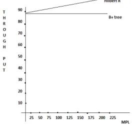
A. B+ Tree versus Hilbert R Tree Performance
The B+ tree can have one of the two fanouts- a high fanout(200 entries/ page) or a low fanout(8 entries/ page). For a comparative study, we consider high fanout case. The system configuration consist of a fixed value for each of the following parameters: the workload, the number of CPUs, the number of disks, the tree fanout, and the buffer pool size. With these parameters in hand, the performance of B+ tree is graphed.
Hilbert R tree, on the other hand, with same parametric conditions show higher performance in high fanout condition. The effectiveness of the technique lies in the fact that it visits minimal number of nodes or less number of files for searching spatial data in map reduce. This tends to minimal search time producing optimized result. Further R tree and its variants can be easily added to any relational database system that supports conventional access methods. Moreover the new structure would work especially well in conjunction with abstract data types and abstract indexes to streamline the handling of spatial data. Hilbert R tree achieves upto 28% saving in the number of pages touched compared to R* tree. The comparison graph varying between Multi-Programmin Level(MPL) and through put using B+ tree and Hilbert R tree is shown.
Figure 4:HIGH FANOUT, SINGLE DISK High fanout:80% Search:1 CPU:1 Disk:200 Bufs
B. Efficient Optimization With Priority R Tree
Priority R tree offers much more efficient space utilization than Hilbert R tree as it completes the searching process of highly prioritized data first. The priority R tree combines K dimensional tree and R tree thus facilitating the storage of spatial data. Hilbert R tree significantly improve performance and decreases insertion complexity while Priority R tree minimizes the overlapping as low as possible. The bulk load performance of Hilbert R tree and priority R tree is graphed below.
TABLE I QUERY PERFORMANCE TABLE
The priority R tree offers two to three times more performance than Hilbert R tree in reading or writing the data blocks. A comparative chart depicting the performance of various indexing trees for different parameters have also been provided, thus motivating the readers to work on the implementation of Hilbert and Priority R tree in a map reduce framework for movement of spatial data.
Figure 5: Bulk loading performance
It is seen from the table that minimal number of files searched and less input – output operations reasonably contribute to efficient optimization of data retrieval in a map reduce environment. It is also evident that Hilbert and Priority R tree shows an effective optimization compared to B tree or B+ tree indexation.
V) CONCLUSIONS AND FUTURE WORK
REFERENCES
[1] Richard McCreadie, Craig Macdonald, Iadh Ounis. Information Processing and Management. In ELSEVIER,2011.
[2] Ralf Hartmut Güting. An Introduction to Spatial Database Systems. In VLDB Journal, 1994.
[3] Lars Arge, Mark de Berg, Herman Haverkort and Ke Yi. The Priority R-Tree: A Practically Efficient and Worst-Case Optimal R-Tree.In SIGMOD,2004.
[4] Karthik Kambatla, Naresh Rapolu, Suresh Jagannathan, Ananth Grama. Asynchronous Algorithms in MapReduce.
[5] Srinivasan, Michael J Carey. Performance of B+ tree concurrency control Algorithm. In VLDB,1993.
[6] Antonin Guttman. R tree: A dynamic indexing structure for spatial searching. In ACM, National science foundation grant and Air force office of scientific research grant,1984.