Improved Multilevel Feedback Queue Scheduling Using Dynamic Time Quantum and Its Performance Analysis

(1)

Improved Multilevel Feedback Queue Scheduling

Using Dynamic Time Quantum and Its Performance

Analysis

H.S. Behera, Reena Kumari Naik, Suchilagna Parida

Department of Computer Science and Engineering, Veer Surendra Sai University of Technology (VSSUT) Burla, Sambalpur, 768018, Odisha,, India

Abstract—Multilevel feedback queue scheduling algorithm allows

a process which is entering to the system to move between several queues. Here, the processes initially does not come with any priority but during scheduling the processes according to their CPU burst time may be shifted to the lower level queues. Here an effective dynamic time slice is used to schedule the processes. As a result we found reduction in turnaround time, average waiting time and better throughput as compared to the previous approaches and hence increase in the overall performance. A control flow diagram is used to describe the sequence of flow of control of the processes with different conditional statements, repetition of the flow structures and case conditions. The algorithm is proposed in such a way that it reduces the starvation of the long processes. An entering process is inserted into the top level queue. When selected, processes in the queue are allocated a relatively small time slice. Upon expiration of time slice the process is moved to lower level queue.

Keywords— CPU burst time, turnaround time,waiting time,throughputs, dynamic time quantum,shifting to lower queues, RR scheduling algorithm.

I. INTRODUCTION

Scheduling is a process of deciding how to allocate resources between different possible tasks. Various types of scheduling algorithms are there such as FCFS, SJF, SRTN, RR etc. In FCFS scheduling algorithm, processes are allowed to get the CPU time according to their arrival time on the ready queue. It is a non-pre emptive algorithm where if a process has a CPU then it runs to completion. SJF scheduling algorithm, the available CPU is assigned to the process that has smallest next CPU burst. In SRTN scheduling algorithm, the scheduler dispatches that ready process which has the shortest expected remaining time to completion. RR scheduling algorithm is the best and most widely used algorithm where the fair share CPU time assigned to the processes based on FCFS basis. Multilevel queue partitions the ready queue into several queues

,

where the processes are permanently assigned to one queue. The processes cannot move between queues. In multilevel feedback queue all the processes entering into the system are assigned to the first queue. Here the processes in

the first queue are scheduled according to the CPU burst time and time quantum selected. The process having CPU burst more than the time quantum are shifted to the next lower level queue. Since, the processes having higher burst time are gradually shifted to the lower level queues so it may suffer from starvation. In this approach, the shorter (highest priority) processes are scheduled using RR scheduling where as the long processes which automatically sink to the lower level queue are served in FCFS order. Until the processes in the higher level queue are completed the scheduler does not allow the process to enter to the next level queue. One drawback of the paper [4] is that the selection of the time quantum by assumption may not perform effectively for all types of processes. So, we have used an effective approach to find the time quantum which results in better performance. The architecture of MLFQ shows a dynamic reduction in turnaround time. The overall performance of the proposed approach is better as compared to previous approaches.

II. RELATED WORK

(2)

average response time. Average response time enters as the input to neural network so that the network obtains a relation between the change of quantum of specified queue with the average response time and with the quantum of other queues and by a change in the quantum of specified queue.

In Paper [8], a different type of analysis has been described which is a combination of both the best case analysis as well as the worst case analysis. The performance is analysed in terms of time complexity. It was also an effective method for better performance of the multilevel feedback queue scheduling. According to paper [10], the multilevel feedback queue scheduling is implemented in Linux kernel. There are many different types of approaches that have already been developed to provide a better idea to improve the performance of multilevel feedback queue in different platforms and by using various methods.

III. PROPOSED APPROACH

In this approach, all the processes are inserted into the first queue and scheduled with the given time slice. The time slices for each queue are selected differently and it gradually increases as the number of queue increases. The time slices are selected based on a new method in order to minimize the turnaround time, waiting time and hence to reduce the starvation of the long processes. The priority of the processes decreases while moving to the lower queues. The processes are scheduled in the first queue using the given time slice. If it is not completed in the current queue then enters into the next queue. Before entering into the next lower level queue the burst time of the processes are updated depending on the time slice. The same procedure is repeated for all the queues which are going to be generated. When the remaining processes reach to the lowest queue the processes are sorted according to their remaining CPU burst time. They are arranged in increasing order according to their values. After that the processes were sent to their respective queues for their total completion. The processes were rescheduled according to the time quantum assigned to the respective queues earlier. The turnaround time, average waiting time and throughput are calculated for the whole process at the end.

III.A. ARCHITECTURE

Here we have taken different types of processes so we found different number of queues in each case. All the processes which are going to be scheduled will enter into Q1. Once the

time quantum expires if a process is not completed then it enters into the next level. The number of levels generated depends upon the time quantum and burst time of the processes. The time quanta calculated are dynamic in nature and they vary for each queue. In the proposed architecture there are 5 queues. The processes which are completed in any queue leave the queue from that level. Here the processes do not have any fixed priority when they enter into the queue. But gradually as they are scheduled the priority is decided

.

The process of scheduling in steps is shown below. Here five queues (Q1, Q2, Q3, Q4 and Q5) are mentioned to describe the

mechanism. If the processes reach at the lowest level queue but are not completed then those remaining processes are to be rescheduled by sending them to the respective queues. This procedure is repeated for the remaining processes till they are completed.

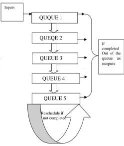
The scheduling mechanism is shown in the below figure:

Figure 1.shows the flow of execution in different level of queues till all the processes get executed.

In the above structure, the processes are inserted into the first queue as input. They are executed and if completed then leave the queue but if not completed then the remaining burst time will enter into next level which is clearly shown in the above diagram. This procedure is repeated up to Q5. When the

processes reach to the lower queue then the remaining burst times were sent to the respective queue according to their values for rescheduling purpose in order to complete the execution

.

III.B.ALGORITHM

Here an effective way was proposed to reduce the starvation of the processes. In the beginning of the scheduling process all the processes are inserted into a queue and it is called as queue1 (Q1). The process having greater burst time than the

assigned time slice goes down. The processes after being

QUEQE 2

QUEUE 3 QUQUE 1

QUEUE 4

QUEUE 5

If completed Out of the

queue as outputs

Inputs

(3)

scheduled in a queue are updated with the new burst time. Here the time at which all processes have finished their execution at one queue is the waiting time for the next queue. When they reach to the lower level queue, the remaining processes are rescheduled by sending them into their respective queue according to their values.

Here we introduced a new approach to find an optimal time quantum. The median and mean of all the processes are calculated using the following formula;

Median= Y (n+1)/2, if n=odd

1/2(Yn/2+ Y (1+n/2)), if n=even

The formula used to calculate the time quantum is mentioned in the pseudo code. So with the calculated time slice the processes are scheduled.

III

.C.

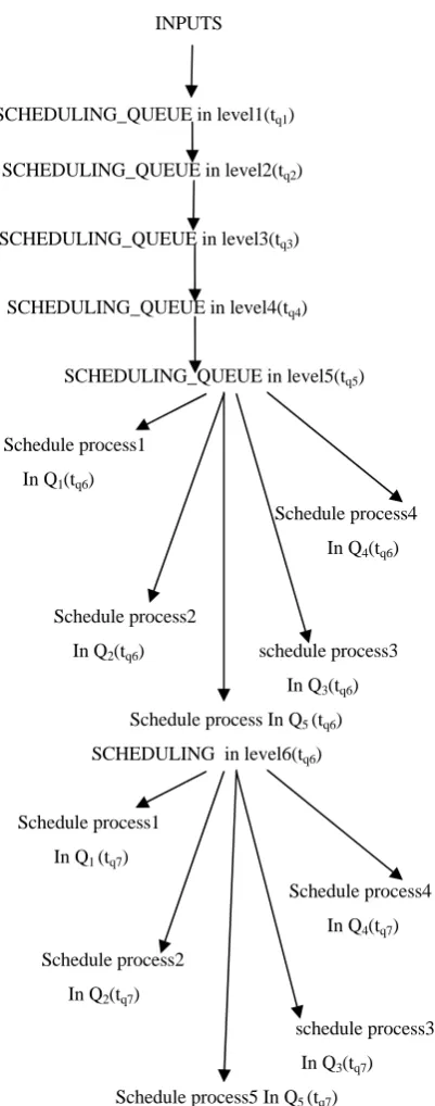
CONTROL FLOW DIAGRAM OFTHE

PROPOSEDALGORITHM

A control flow diagram (CFD) describes the sequence of flow of control of process or program. It can consist of a subdivision to show sequential steps, with different conditional statements, repetitions and case conditions. Here we have taken 5 queues (Q1, Q2, Q3, Q4 and Q5).

If any process does not complete its execution within these queues and reaches to the lowest queue i.e. Q5 then the

remaining processes are to be rescheduled in their respective queues. The processes are arranged according to their remaining CPU burst time and send them to their respective queues. The processes are in increasing or decreasing order and the process having minimum burst time is sent to Q1 and

PSEUDO CODE OF THE PROPOSED ALGORITHM:

1. Qm: number of queue, where m represent the number from 1, 2, 3…..

n=no. of processes

Yn= position of the nthprocess

bt [i]: burst time of ith process

rbt [i]: remaining burst time of ith process

tq =time quantum,

Initialize: m=1, i=1, avg tat=0

2. Insert the processes p[i] where i=1 to n to Q1.

3. Calculate the tq

For (m=1 to 5)

While (ready queue! =NULL) {

tq1=|Mean-Median|/3;

tq2=2*tq1;

tq3=2*tq2;

}/* A recursive method is used to calculate tq

For Q1 to Q5*/

4. Assign tq to each process in the Qm for each process

p [i] where i=1 to n. P [i] ->tq

5. If (bt [i]>=tq)

{

Qm+1bt[i]-tq

// rbt[i] of P[i] after the tq used is assigned to next

queue }

Else Qm-> bt[i]

/*bt[i] is used in the same queue hence process

Expires at the same level*/

6. Calculate the waiting time for Qm+1 at each Qm.

7. If a new queue arrives

Update the values m and n and go to step 3.

8. If (m>5) /* Here, we have considered the number of queues as 5.*/

{

Arranged the rbt [i] of processes in increasing order.

Reschedule the remaining processes in their respective queues according to their values.

/* least remaining process will go to Q1 and next up

to Q5.*/

}

9. Calculate tat, avg waiting time & throughput at the end.

(4)

next process to Q2 and in the same way processes are assigned

up to Q5 so that Q5 must get the process with highest

remaining burst time.The same procedure repeats till all the processes have finished their execution.

INPUTS

SCHEDULING_QUEUE in level1(tq1)

Schedule process1

In Q1(tq6)

Schedule process4

In Q4(tq6)

Schedule process2

In Q2(tq6) schedule process3

In Q3(tq6)

Schedule process In Q5 (tq6)

SCHEDULING in level6(tq6)

Schedule process1

In Q1 (tq7)

Schedule process4

In Q4(tq7)

Schedule process2

In Q2(tq7)

schedule process3 In Q3(tq7)

Schedule process5 In Q5 (tq7)

Figure 2.Control Flow Diagram showing the scheduling process. The process of execution repeats till all the processes are finished within their given burst times. Here the order of time quanta is

tq1 < tq2 <tq3 <tq4 <tq5 <tq6 <tq7

III.D.FLOW CHART OF THE PROPOSED ALGORITHM

Yes

No

Yes

No

Yes

Figure 3.Representing the flow of sequence of processes from one queue to next.

Start

Input

Assigned all processes to While

(m<=5)

Is Ready queue= null?

Tq=

| Mean- Median|/3

P[i]tq

Is bt >tq

?

Rbt=bt-tq

Qm tq

Qm+1rbt

Is m>5 ?

Sort rbt[i]

Calculate avg waiting time, and throughput

(5)

IV.EXPERIMENTALANALYSIS

The proposed algorithm was elaborated with the following processes. There are five processes with different arrival time and CPU Burst time. These processes are to be scheduled according to the given time slice for each queue. The time slice gradually increases as the queues go down to the lower level. We have taken different time slice for respective queues from Q1 to Q5. The turnaround time was calculated for the whole

scheduling mechanism.

IV.A.GANTTCHART

A Gantt chart is a type of bar chart ,that illustrates a process schedule. Gantt charts differentiate the start and finish time of the processes in the queue . This chart also shows the dependency (i.e., precedence network) relationships between different queues which is shown in the Multilevel Feedback Queue.

Following example elaborates the performance enhancing scenario with suitable Gantt chart and result.

Table 1: TEST CASE INPUT:

(Five processes with CPU burst times and arrival times) Processes CPU burst time Arrival time

P1 421 1 P2 551 3 P3 299 7 P4 326 8 P5 346 9 According to the proposed algorithm the time quanta are calculated as follows for different queues;

tq1=|mean-median|/3=|389-346|/3=14

tq2=2*tq1=2*14=28

tq3=2*tq2=2*28=56

tq4=2*tq3=2*56=112

tq5=2*tq4=2*112=224

The above processes are to be scheduled through different queues with the assigned time quantum for each queue. The time at which the current queue completes is the waiting time for the next queue. The first arrival time here is 1.The scheduling process is as follows:

The waiting time for the Q1 is T1=1;

Queue1:-

P1 P2 P3 P4 P5 1 15 29 43 57 71

The waiting time for the next queue is same as the time at which the processes in the first queue are completed. Because the control of execution enters into the second queue if and only if the first queue is executed. Hence the waiting time for Q2 is T2=71;

Queue2:-

P1 P2 P3 P4 P5 71 99 127 155 183 211 The waiting time for Q3 is T3=211;

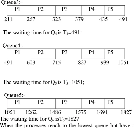
Queue3:-

P1 P2 P3 P4 P5 211 267 323 379 435 491 The waiting time for Q4 is T4=491;

Queue4:-

P1 P2 P3 P4 P5 491 603 715 827 939 1051

The waiting time for Q5 is T5=1051;

Queue5:-

P1 P2 P3 P4 P5 1051 1262 1486 1575 1691 1827 The waiting time for Q6 isT6=1827

When the processes reach to the lowest queue but have not completed then the remaining CPU burst time of each process are calculated and range the values in increasing or decreasing order .Rescheduled the processes by sending them into their required respective queues. The process having least burst time is send to Q1 and the next process to Q2. In the same

manner all processes have been sent to different queues according to their values. Q5 must have the process with

highest remaining burst time. The same procedure is repeated till all the processes get executed.

Here in this above example P2 is only remaining with burst time of 117 so it is sent to Q5 for completion.

T6=1827

Queue 5

P2

1827 1944

Here the turnaround time calculated by the proposed approach is 1944nm.

(6)

Table 2(a): FIRST TEST CASE INPUT:

(Five processes with different arrival times and CPU burst times)

Table 2(b): FIRST TEST CASE OUTPUT: algorithms Turn around time Average waiting time throughput Power MLFQ 2944 761 0.00016

EMLFQ 2736 761 0.00018 Proposed approach 2525 666 0.00019

Table 3(a): SECOND TEST CASE INPUT: (Five processes with different arrival times and CPU burst times)

PROCESSES CPU BURST TIME ARRIVAL TIME

P1 421 1

P2 551 4

P3 299 6

P4 326 9

P4 346 10

Table 3(b): SECOND TEST CASE OUTPUT:

Table 4(a): THIRD TEST CASE INPUT:

(Five processes with different arrival times and CPU burst times)

PROCESSES CPU BURST TIME ARRIVAL TIME

P1 821 1

P2 951 2

P3 699 8

P4 726 11 P5 746 14 Table 4(b): THIRD TEST CASE OUTPUT:

algorithms Turn around time Average waiting time Throughput Power MLFQ 4068 761 0.00012

EMLFQ 3969 761 0.00012 Proposed approach 3066 666 0.00016

In all the above test cases the calculated turnaround time, average waiting time & throughput are better than previous MLFQ papers.

III.B. PERFORMANCE ANALYSIS

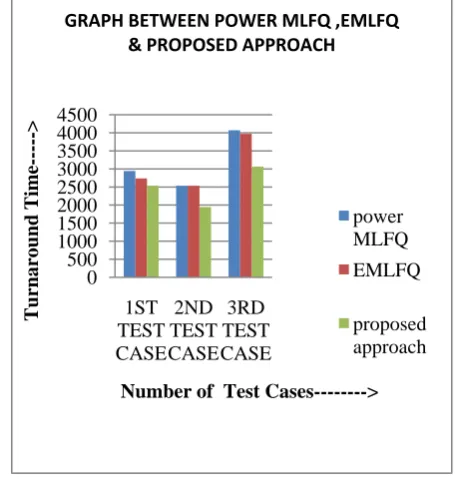
Here the performance of the proposed approach was compared with the previous papers by taking different test cases and represented below in the form of graph. The graph shows the turnaround time, average waiting time and throughput along the Y-axis and the number of test cases along the X-axis. The turnaround time, average waiting time and throughput in the proposed algorithm are better in all the cases than previous papers. 0 500 1000 1500 2000 2500 3000 3500 4000 4500 1ST TEST CASE 2ND TEST CASE 3RD TEST CASE Turnaround Time--->

Number of Test Cases--->

GRAPH BETWEEN POWER MLFQ ,EMLFQ

& PROPOSED APPROACH

power MLFQ EMLFQ proposed approach

Figure 4.turnaround time of various proposed approaches for 1st test case, 2nd test case and 3rd test case are shown.

0 100 200 300 400 500 600 700 800 1ST TEST CASE 2ND TEST CASE 3RD TEST CASE Av g wa it in g Ti m e ‐‐‐‐‐ >

Number of Test Cases--->

GRAPH BETWEEN POWER MLFQ

,EMLFQ & PROPOSED APPROACH

power MLFQ EMLFQ

proposed a pproa ch

Figure 5.Average waiting time of the queues at each level of various proposed approaches for 1st test case, 2nd test case &

3rd test case are shown. PROCESSES CPU BURST TIME ARRIVAL TIME

P1 621 1

P2 751 3

P3 499 6

P4 526 9

P5 546 10

Algorithms Turnaround time

Average waiting

time

throughput

Power MLFQ 2535 662 0.00019

EMLFQ 2535 662 0.00019

(7)

0 0.00005 0.0001 0.00015 0.0002 0.00025 0.0003

1ST TEST CASE

2ND TEST CASE

3RD TEST CASE

Thr

o

ug

hput

‐‐‐‐‐

>

Number of Test Cases‐‐‐‐‐‐‐‐>

GRAPH BETWEEN POWER MLFQ ,EMLFQ

& PROPOSED APPROACH

power MLFQ EMLFQ

proposed approach

Figure 6.throughput of various proposed approaches for 1st test case, 2nd test case and 3rd test case are shown.

V.CONCLUSIONANDFUTUREWORK

An effective study was made to assign various processes into different queues and the flow of control was clearly distinguished from one queue to another with the help of the control flow diagram. The starvation of the long process is reduced in the proposed approach.

It was also noted that the number of queues and quantum of each queue affect the response time directly. Hence, a better and optimal time quantum was introduced. As a result reduction in the turnaround time of the scheduling process in Multilevel Feedback Queue Scheduling was achieved. The waiting time for each queue has also been reduced. As the turnaround time and waiting time decreases, the execution becomes faster.

Here we found less turnaround time , average waiting time and throughput than the previous proposed algorithm so

we can conclude that this proposed approach shows a better result. Hence the overall performance of the multilevel feedback scheduling is better than the previous approaches. This algorithm can be used on time sharing systems and distributed systems in an effective way that the research is still being continued in these fields.

REFERENCES

1. Baney, Jim and Livny, Miron (2000),” Managin NetworkResources in Condor”, 9th_{IEEE Proceedings of the International Symposium on High}

Performance Distributed Computing, Washington, DC, USA.

2. Parvar, Mohammad R.E, Parvar, M.E. and Safari, Saeed (2008),”A Starvation Free IMLFQ Scheduling Algorithm Based on Nueral Network”, International Journal of Computational Intelligence Research ISS 0973-1873 Vol.4, No.1 pp.27-36.

3. Wolski, Rich, Nurmi, Daniel and Brevik, Jhon (2007),” An Analysis of Availability Distributions in Condor”, IEEE, University of California, Santa Barbara.

4. Becchetti, L., Leonardi, S. and Marchetti S.A. (2006),” Average-Case and Smoothed Competitive Analysis of the Multilevel Feedback Algorithm” Mathematics of Operation Research Vol.31, No.1, February, pp.85-108.

5. Litzkow, Micheal J., Linvey, Miron and Mutka, Matt W. (1988),” Condor –A Hunter of Idle Workstations” IEEE, Department of Computer Sciences, University of Wisconsin, Madison.

6. Abawajy, Jemal H. (2002),”Job Scheduling Policy for High Throughput Computing Environments”, Ninth IEEE International Conferences on Parallel and Distributed Systems, Ottawa, Ontario, Canada.

7. Liu, Chang, Zhao, Shawn and Liu, Fang (2009), “An Insight into the architecture of Condor-a Distributed Scheduler”, IEEE, Beijing, China.

AUTHOR’S BIOGRAPHY

1. Dr. H. S. Behera is currently working as a Faculty in Dept. of Computer Science and Engineering, Veer Surendra Sai University of Technology (VSSUT), Burla, Sambalpur, 768018, Odisha, India. His areas of interest include Distributed Systems, Data Mining, and Soft Computing.

2. Reena Kumari Naik is a final year B.Tech student in Dept. of Computer Science and Engineering, Veer Surendra Sai University of Technology (VSSUT), Burla, Sambalpur, 768018, Odisha, India.