Dalitz Plot Analysis of Three-body Charmonium Decays at BABAR

Dalitz Plot Analysis of Three-body Charmonium Decays at

BA

B

AR

Antimo Palano1,3,⋆

1_{INFN and University of Bari, Via Orabona 4, 70125 Bari, Italy}

Abstract. We present results on the measurement of the I=1/2KπS-wave through a model independent partial wave analysis ofηcdecays toKS0K

+_π−_andK+_K−_π0_produced

in two-photon interactions. We also perform Dalitz plot analyses of the J/ψdecays to π+_π−_π0_,K+_K−_π0_andK0

SK

±_π∓_{produced in the initial state radiation process.}

1 Introduction

Charmonium decays can be used to obtain new information on light meson spectroscopy. Ine+_e− interactions, samples of charmonium decays can be obtained using different processes.

• In two-photon interactions we select events in which thee+ _ande− _{beam particles are scattered} at small angles and remain undetected. Only resonances withJPC _{= 0}±+_,2±+_,3++_,4±+_{.... can be} produced.

• In the Initial State Radiation (ISR) process, we reconstruct events having a (mostly undetected) fast forwardγIS Rand, in this case, onlyJPC =1−−states can be produced.

2 Study of

η

→

K

K

¯

π

The BaBar Dalitz plot analysis of theηc→ K+K−ηandηc →K+K−π0has provided the unexpected

observation ofK∗

0(1430) → Kη[1]. We also find that the ηc three-body hadronic decays proceed almost entirely through the intermediate production of scalar meson resonances.

We study the reactions [2]

γγ → K_S0K+_π−

, γγ → K+_K−_π0 .

In the following, details on events reconstruction will be given only for theK0_SK+_π−

final state. We select events having only four tracks. Since two-photon events balance the transverse momentum, we requirepT, the transverse momentum of theKS0K

+_π−

system with respect to the beam axis, to be pT <0.08GeV/c. We also defineM2rec ≡(pe+_e−−p_rec)2, where p_e+_e−is the four-momentum of the

initial state andprecis the four-momentum of theKS0K

+_π−_{system and remove ISR events requiring}

M2

rec>10GeV2/c4. TheKS0K

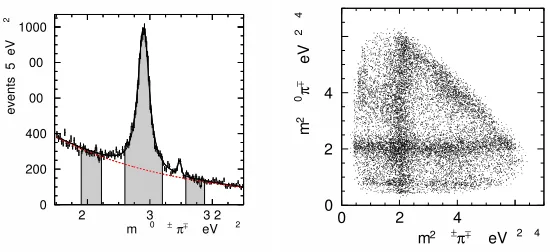
+_π−_{mass spectrum in theη}

cmass regions is shown in Fig. 1(left) and

theηcDalitz plot is shown in Fig. 1(right). The Dalitz plot is dominated by the presence of horizontal

and vertical uniform bands at the position of theK∗

0(1430) resonance. The corresponding distributions forηc→K+K−π0can be found in Ref. [1] and present similar features.

2

eV ±

π

± 0

m

2 3 3 2

2

events5eV

0 200 400 00 00 1000

4 2

eV

± π

±

2

m

0 2 4

4

2

eV

±

π

0

2

m

0 2 4

Figure 1.(left)K0

SK

+_π−_{mass spectrum in two-photon interactions and (right) theη}

c→KS0K

+_π−_{Dalitz plot.}

The ηc signal regions contain 12849 events with (64.3±0.4)% purity for ηc → KS0K

+_π− _and

6494 events with (55.2±0.6)% purity forηc → K+K−π0. The backgrounds below theηcsignals are

estimated from the sidebands. We observe asymmetricK∗’s in the background to theηc→ KS0K +_π−

final state due to interference between I=1 and I=0 contributions.

3 Dalitz plot Analysis of

η

→

K

K

¯

π

We perform unbinned maximum likelihood fits using the Isobar model [3] and Model Independent Partial Wave Analysis (MIPWA) [4]. In the MIPWA theKπmass spectrum is divided into 30 equally spaced mass intervals 60 MeV/c2 wide and for each bin we add to the fit two new free parameters, the amplitude and the phase of theKπS-wave (constant inside the bin). We also fix the amplitude to 1.0 and its phase toπ/2 in an arbitrary interval of the mass spectrum (bin 11 which corresponds to a mass of 1.45 GeV/c2). The number of additional free parameters is therefore 58. Due to isospin conservation in the decays, amplitudes are symmetrized with respect to the twoKπdecay modes. TheK∗

2(1420),a0(980),a0(1400),a2(1310), ... contributions are modeled as relativistic Breit-Wigner functions multiplied by the corresponding angular functions. Backgrounds are fitted separately and interpolated into theηcsignal regions. The fits improves when an additional high massa0(1950)→ KK¯ I=1 resonance is included with free parameters in bothηcdecay modes. The weighted average of

the two measurement is:m(a0(1950))=1931±14±22 MeV/c2,Γ(a0(1950))=271±22±29 MeV. The statistical significances for thea0(1950) effect (including systematics) are 2.5σforηc→KS0K

+_π−

and 4.0σforηc→K+K−π0.

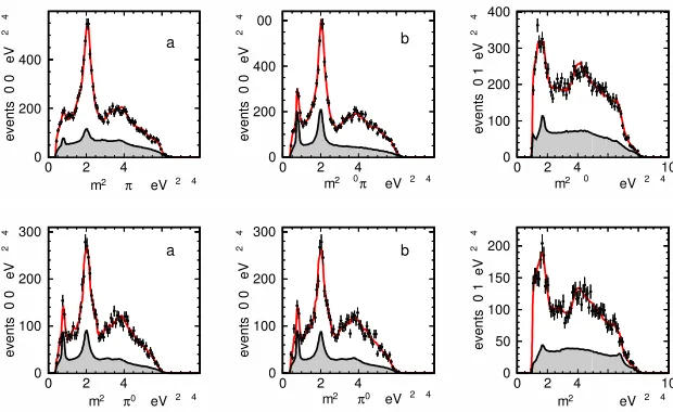
The Dalitz plot projections with fit results forηc → KS0K +_π−

andηc → K+K−π0 are shown in

Fig. 2. The fitted fractions and phases are given in Table 1. We observe a good description of the data. We note that theK∗_{(892) contributions arise entirely from background.}

In comparison, the isobar model gives a worse description of the data, withχ2_/N

cells=457/254=

1.82 andχ2_/N

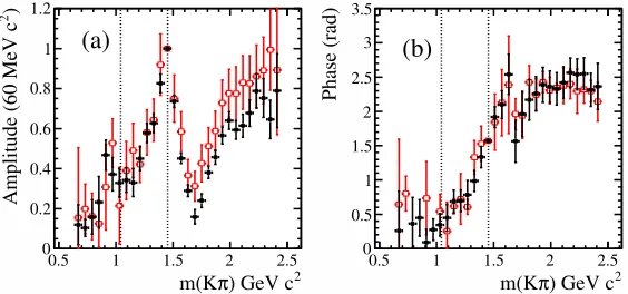
cells = 383/233 = 1.63 respectively for the twoηcdecay modes. The resulting Kπ

S-wave amplitude and phase for the two ηc decay modes is shown in Fig. 3. We observe a clear

K₀∗(1430) resonance signal with the corresponding expected phase motion. At high mass we observe the presence of the broad K∗₀(1950) contribution with good agreement between the two ηc decay

modes. Comparing with LASS [5] and E791 [4] experiments we note that phases before the Kη′

2 eV ± π ± 0 m

2 3 3 2

2 events5eV 0 200 400 00 00 1000 4 2 eV ± π ± 2 m

0 2 4

4 2 eV ± π 0 2 m 0 2 4

Figure 1.(left)K0

SK

+_π−_{mass spectrum in two-photon interactions and (right) theη}

c→K0SK

+_π−_{Dalitz plot.}

The ηc signal regions contain 12849 events with (64.3±0.4)% purity for ηc → KS0K

+_π− _and

6494 events with (55.2±0.6)% purity forηc → K+K−π0. The backgrounds below theηcsignals are

estimated from the sidebands. We observe asymmetricK∗’s in the background to theηc→ KS0K +_π−

final state due to interference between I=1 and I=0 contributions.

3 Dalitz plot Analysis of

η

→

K

K

¯

π

We perform unbinned maximum likelihood fits using the Isobar model [3] and Model Independent Partial Wave Analysis (MIPWA) [4]. In the MIPWA theKπmass spectrum is divided into 30 equally spaced mass intervals 60 MeV/c2 wide and for each bin we add to the fit two new free parameters, the amplitude and the phase of theKπS-wave (constant inside the bin). We also fix the amplitude to 1.0 and its phase toπ/2 in an arbitrary interval of the mass spectrum (bin 11 which corresponds to a mass of 1.45 GeV/c2). The number of additional free parameters is therefore 58. Due to isospin conservation in the decays, amplitudes are symmetrized with respect to the two Kπdecay modes. TheK∗

2(1420),a0(980),a0(1400),a2(1310), ... contributions are modeled as relativistic Breit-Wigner functions multiplied by the corresponding angular functions. Backgrounds are fitted separately and interpolated into theηcsignal regions. The fits improves when an additional high massa0(1950)→ KK¯ I=1 resonance is included with free parameters in bothηcdecay modes. The weighted average of

the two measurement is:m(a0(1950))=1931±14±22 MeV/c2,Γ(a0(1950))=271±22±29 MeV. The statistical significances for thea0(1950) effect (including systematics) are 2.5σforηc→KS0K

+_π−

and 4.0σforηc→K+K−π0.

The Dalitz plot projections with fit results forηc → KS0K +_π−

andηc → K+K−π0 are shown in

Fig. 2. The fitted fractions and phases are given in Table 1. We observe a good description of the data. We note that theK∗_{(892) contributions arise entirely from background.}

In comparison, the isobar model gives a worse description of the data, withχ2_/N

cells=457/254=

1.82 andχ2_/N

cells = 383/233 = 1.63 respectively for the two ηc decay modes. The resultingKπ

S-wave amplitude and phase for the two ηc decay modes is shown in Fig. 3. We observe a clear

K₀∗(1430) resonance signal with the corresponding expected phase motion. At high mass we observe the presence of the broad K₀∗(1950) contribution with good agreement between the two ηc decay

modes. Comparing with LASS [5] and E791 [4] experiments we note that phases before the Kη′

threshold are similar, as expected from Watson [6] theorem but amplitudes are very different.

4 2 eV π 2 m

0 2 4

4 2 events00eV 0 200 400 a 4 2 eV π 0 2 m

0 2 4

4 2 events00eV 0 200 400 00 b 4 2 eV 0 2 m

0 2 4 10

4 2 events01eV 0 100 200 300 400 4 2 eV 0 π 2 m

0 2 4

4 2 events00eV 0 100 200 300 a 4 2 eV 0 π 2 m

0 2 4

4 2 events00eV 0 100 200 300 b 4 2 eV 2 m

0 2 4 10

4 2 events01eV 0 50 100 150 200

Figure 2. (top)ηc →KS0K

+_π−_{and (bottom)η}

c →K+K−π0 Dalitz plots projections. The superimposed curves are from the fit results. Shaded is contribution from the interpolated background.

Table 1.Results from theηc→KS0K

±_π∓_andη

c→K+K−π0MIPWA. Phases are determined relative to the (KπS-wave)Kamplitude which is fixed toπ/2 at 1.45 GeV/c2_.

ηc→KS0K

±_π∓ _η

c→K+K−π0

Amplitude Fraction (%) Phase (rad) Fraction (%) Phase (rad)

(KπS-wave)K 107.3±2.6±17.9 fixed 125.5±2.4±4.2 fixed

a0(980)π 0.8±0.5± 0.8 1.08±0.18±0.18 0.0±0.1±1.7

-a0(1450)π 0.7±0.2± 1.4 2.63±0.13±0.17 1.2±0.4±0.7 2.90±0.12±0.25

a0(1950)π 3.1±0.4± 1.2 −1.04±0.08±0.77 4.4±0.8±0.8 −1.45±0.08±0.27

a2(1320)π 0.2±0.1± 0.1 1.85±0.20±0.20 0.6±0.2±0.3 1.75±0.23±0.42

K∗

2(1430)K 4.7±0.9± 1.4 4.92±0.05±0.10 3.0±0.8±4.4 5.07±0.09±0.30

Total 116.8±2.8±18.1 134.8±2.7±6.4

−2 logL −4314.2 −2339

χ2_{/Ncells 301/254=1.17 283.2/233=1.22}

4 Dalitz plot analysis of

J

/ψ

→

π

π

π

,

J

/ψ

→

K

K

π

and

J

/ψ

→

K

K

±

π

Only a preliminary result exists, to date, on a Dalitz-plot analysis ofJ/ψdecays toπ+_π−_π0_{[7]. While} large samples ofJ/ψdecays exist, some branching fractions remain poorly measured. BES III exper-iment has performed an angular analysis ofJ/ψ → K+_K−_π0_{. The analysis requires the presence of a} broadJPC₌₁−−_{state in theK}+_K−_{threshold region, which is interpreted as a multiquark state [8].}

We study the following reactions:

2

) GeV c

π

m(K

0.5 1 1.5 2 2.5

)

2

Amplitude(60MeVc

0 0.2 0.4 0.6 0.8 1 1.2

(a)

2

) GeV c

π

m(K

0.5 1 1.5 2 2.5

Phase(rad)

0 0.5 1 1.5 2 2.5 3 3.5

(b)

Figure 3. TheI =1/2KπS-wave amplitude (a) and phase (b) fromηc→ K0SK

+_π−_{(solid (black) points) and}

ηc→K+K−π0(open (red) points); only statistical uncertainties are shown. The dotted lines indicate theKηand Kη′_thresholds.

whereγISRindicate the (mostly undetected) ISR photon. We computeMrec2 ≡(pe−+p_e+−p_h+−p_h−−

ph0)2, wherehindicates the three hadrons in the final states. This quantity should peak near zero for ISR events. We select events in the ISR region by requiring|Mrec2 | < 2GeV2/c4 for the reactions involving aπ0and|M2rec|<1.5GeV2/c4for the reaction with aKS0. We fit the mass spectra using the

Monte Carlo resolution functions described by a Crystal Ball+Gaussian functions. We obtain 19560

±164 events forJ/ψ → π+_π−_π0_{with (91.3±0.2)% purity, 2002±48 forJ/ψ → K}+_K−_π0 _with (88.8±0.7)% purity, and 3694±64 with 93.1±0.4 purity for J/ψ → K0

SK

±_π∓_{. The efficiency is}

mapped and fitted on the (m(h+_h−_),cosθ

h) plane, whereθh is theh+helicity angle in the J/ψrest

frame. To obtain the measurements of the relative branching fractions, we correct yields by weighting each event by the inverse of the efficiency and perform background subtraction by assigning negative weights to events theJ/ψsidebands regions. We measure the ratio

R1=

B(J/ψ → K+K−π0)

B(J/ψ → π+_π−_π0₎ =0.120±0.003(stat)±0.009(sys), (1)

where many systematic uncertainties cancel out due to the similar event topology of theJ/ψdecay modes. The PDG reportsB(J/ψ → π+_π−_π0_{) =(2.11±0.07)×10}−2_{, while the branching fraction}

B(J/ψ → K+_K−_π0_{) has been measured by Mark II [9] using 25 events, to be (2.8±0.8)×10}−3_. These values give a ratioRPDG

1 =0.133±0.038, in agreement with our measurement. Using a similar procedure and correcting correcting for unseenK0

S decay modes, we compute the relative branching

fraction

R2=

B(J/ψ→K0

SK ±_π∓₎

B(J/ψ→π+_π−_π0₎ =0.265±0.005(stat)±0.021(sys). (2)

The branching fractionB(J/ψ→ K0

SK ±_π∓

) has been measured by Mark I [10], using 126 events, to be (26±7)×10−4_{. Using the above measurements we obtain an estimate ofR}PDG

2 =0.123±0.033, which deviates by 3.6σfrom our measurement.

5

J

/ψ

→

π

π

π

Dalitz plot analysis

2

) GeV c

π

m(K

0.5 1 1.5 2 2.5

)

2

Amplitude(60MeVc

0 0.2 0.4 0.6 0.8 1 1.2

(a)

2

) GeV c

π

m(K

0.5 1 1.5 2 2.5

Phase(rad)

0 0.5 1 1.5 2 2.5 3 3.5

(b)

Figure 3. TheI =1/2KπS-wave amplitude (a) and phase (b) fromηc→ KS0K

+_π−_{(solid (black) points) and}

ηc→K+K−π0(open (red) points); only statistical uncertainties are shown. The dotted lines indicate theKηand Kη′_thresholds.

whereγISRindicate the (mostly undetected) ISR photon. We computeMrec2 ≡(pe−+p_e+−p_h+−p_h−−

ph0)2, wherehindicates the three hadrons in the final states. This quantity should peak near zero for ISR events. We select events in the ISR region by requiring|Mrec2 | < 2GeV2/c4 for the reactions involving aπ0and|M2rec|<1.5GeV2/c4for the reaction with aKS0. We fit the mass spectra using the

Monte Carlo resolution functions described by a Crystal Ball+Gaussian functions. We obtain 19560

±164 events forJ/ψ → π+_π−_π0 _{with (91.3±0.2)% purity, 2002±48 forJ/ψ → K}+_K−_π0_with (88.8±0.7)% purity, and 3694±64 with 93.1±0.4 purity for J/ψ → K0

SK

±_π∓_{. The efficiency is}

mapped and fitted on the (m(h+_h−_),cosθ

h) plane, whereθh is theh+ helicity angle in theJ/ψrest

frame. To obtain the measurements of the relative branching fractions, we correct yields by weighting each event by the inverse of the efficiency and perform background subtraction by assigning negative weights to events theJ/ψsidebands regions. We measure the ratio

R1=

B(J/ψ → K+K−π0)

B(J/ψ → π+_π−_π0₎ =0.120±0.003(stat)±0.009(sys), (1)

where many systematic uncertainties cancel out due to the similar event topology of the J/ψdecay modes. The PDG reportsB(J/ψ → π+_π−_π0_{) =(2.11±0.07)×10}−2_{, while the branching fraction}

B(J/ψ → K+_K−_π0_{) has been measured by Mark II [9] using 25 events, to be (2.8±0.8)×10}−3_. These values give a ratioRPDG

1 =0.133±0.038, in agreement with our measurement. Using a similar procedure and correcting correcting for unseenK0

S decay modes, we compute the relative branching

fraction

R2=

B(J/ψ→K0

SK ±_π∓₎

B(J/ψ→π+_π−_π0₎ =0.265±0.005(stat)±0.021(sys). (2)

The branching fractionB(J/ψ→ K0

SK ±_π∓

) has been measured by Mark I [10], using 126 events, to be (26±7)×10−4_{. Using the above measurements we obtain an estimate ofR}PDG

2 =0.123±0.033, which deviates by 3.6σfrom our measurement.

5

J

/ψ

→

π

π

π

Dalitz plot analysis

The Dalitz plot forJ/ψ → π+π−π0is shown in Fig. 4 and is dominated by threeρ(770)π contribu-tions. We perform a Dalitz plot analysis using the isobar model with amplitudes described by Zemach

4 2

eV

0 π π 2

m

0 2 4

4

2

eV

0

π

π

2

m

0 2 4

Figure 4.J/ψ → π+_π−_π0_{Dalitz plot.}

tensors [11, 12] and the Veneziano model [13]. The results from the Dalitz analysis are tabulated in Table 2 and fit projections are shown in fig. 5. The Veneziano model deals with trajectories rather

4 2

eV

π π

2

m

0 2 4 10

4

2

events01eV

0 500 1000

4 2

eV

0

π

±

π

2

m

0 2 4 10

4

2

events01eV

0 500 1000 1500 2000

Figure 5.(left)m2_(π+_π−_{) and (right)m}2_(π±_π0_{) forJ/ψ → π}+_π−_π0_{. Shaded is the background interpolated from} J/ψsidebands.

than single resonances. The complexity of the model is related ton, the number of Regge trajectories included in the fit which requires n=7, described by 19 free parameters.

Figure 8(a) shows the combinatorial cosθπhelicity angle vs.m(ππ). Figure 8 also shows them(ππ)

mass projection for|cosθπ|<0.2 for the isobar model fit (b) and Veneziano model (c). The helicity

Table 2.Results from the Dalitz-plot analysis of theJ/ψ → π+_π−_π0_{channel. When two uncertainties are}

given, the first is statistical and the second systematic. The error on the amplitude is only statistical.

Final state Amplitude Isobar fraction (%) Phase (radians) Veneziano fraction (%)

ρ(770)π 1. 114.2±1.1 ±2.6 0. 133.1±3.3

ρ(1450)π 0.513±0.039 10.9±1.7 ±2.7 −2.63±0.04±0.06 0.80±0.27

ρ(1700)π 0.067±0.007 0.8±0.2 ±0.5 −0.46±0.17±0.21 2.20±0.60

ρ(2150)π 0.042±0.008 0.04±0.01±0.20 1.70±0.21±0.12 6.00±2.50

ω(783)π0 _{0.013±0.002 0.08±0.03±0.02 2.78±0.20±0.31}

ρ3(1690)π 0.40±0.08

Sum 127.8±2.0±4.3 142.5±2.8

χ2/ν 687/519=1.32 596/508=1.17

2

e c

π π

m

1 2 3

π

θ

os

1

−

5

−

5 1

a

2

e c

π π

m

1 2 3

2

events003eV

1 1

2

1

3

1 b

2

e c

π π

m

1 2 3

2

events003eV

1 1

2

1

3

1 c

Figure 6.(a) Binned scatter diagram of cosθπ3vs m(π1π2). (b), (c)ππmass projection in the|cosθπ|<0.2 region for all the threeππcharge combinations. The horizontal lines in (a) indicate the cosθπselection. The dashed line in (b) is the result from the fit with only theρ(770)πamplitude. The fit in (b) uses the isobar model and the shaded histogram shows the background distribution estimated from theJ/ψsidebands. The fit in (c) uses the Veneziano model.

6

J

/ψ

→

K

K

π

and

J

/ψ

→

K

K

π

Dalitz plot analyses

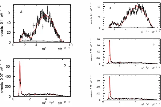
We perform a Dalitz-plot analysis ofJ/ψ → K+K−π0in theJ/ψsignal region. Figure 7(left) shows the Dalitz plot for theJ/ψsignal region and Fig. 8(left) shows the Dalitz plot projections. We observe that the decay is dominated by theK∗₍₈₉₂₎±_K∓_{amplitude. We also observe a diagonal band which} we tentatively attribute to theρ(1450)0_π0_{amplitude. We fit theJ/ψ → K}+_K−_π0_{Dalitz plot using the} isobar model. The results from the fit are given in Table 3 and fit projections are shown in Fig. 8(left). The Dalitz analysis is describing well theK+_K−_{threshold region and therefore we assign the broad} enhancement in theK+_K−_{mass spectrum to the presence of theρ(1450) resonance: the present data} do not require the presence of an exotic contribution.

We perform a similar Dalitz plot analysis of J/ψ → K_S0K±π∓ in the J/ψsignal region. Fig-ure 7(right) shows the Dalitz plot for theJ/ψsignal region and Fig. 8(right) shows the Dalitz plot projections. We fit theJ/ψ → KS0K

±_π∓

Table 2.Results from the Dalitz-plot analysis of theJ/ψ → π+_π−_π0_{channel. When two uncertainties are}

given, the first is statistical and the second systematic. The error on the amplitude is only statistical.

Final state Amplitude Isobar fraction (%) Phase (radians) Veneziano fraction (%)

ρ(770)π 1. 114.2±1.1 ±2.6 0. 133.1±3.3

ρ(1450)π 0.513±0.039 10.9±1.7 ±2.7 −2.63±0.04±0.06 0.80±0.27

ρ(1700)π 0.067±0.007 0.8±0.2 ±0.5 −0.46±0.17±0.21 2.20±0.60

ρ(2150)π 0.042±0.008 0.04±0.01±0.20 1.70±0.21±0.12 6.00±2.50

ω(783)π0 _{0.013±0.002 0.08±0.03±0.02 2.78±0.20±0.31}

ρ3(1690)π 0.40±0.08

Sum 127.8±2.0±4.3 142.5±2.8

χ2/ν 687/519=1.32 596/508=1.17

2

e c

π π

m

1 2 3

π θ os 1 − 5 − 5 1 a 2 e c π π m

1 2 3

2 events003eV 1 1 2 1 3 1 b 2 e c π π m

1 2 3

2 events003eV 1 1 2 1 3 1 c

Figure 6.(a) Binned scatter diagram of cosθπ3vs m(π1π2). (b), (c)ππmass projection in the|cosθπ|<0.2 region for all the threeππcharge combinations. The horizontal lines in (a) indicate the cosθπselection. The dashed line in (b) is the result from the fit with only theρ(770)πamplitude. The fit in (b) uses the isobar model and the shaded histogram shows the background distribution estimated from theJ/ψsidebands. The fit in (c) uses the Veneziano model.

6

J

/ψ

→

K

K

π

and

J

/ψ

→

K

K

π

Dalitz plot analyses

We perform a Dalitz-plot analysis ofJ/ψ → K+K−π0in theJ/ψsignal region. Figure 7(left) shows the Dalitz plot for theJ/ψsignal region and Fig. 8(left) shows the Dalitz plot projections. We observe that the decay is dominated by theK∗₍₈₉₂₎±_K∓_{amplitude. We also observe a diagonal band which} we tentatively attribute to theρ(1450)0_π0_{amplitude. We fit theJ/ψ → K}+_K−_π0_{Dalitz plot using the} isobar model. The results from the fit are given in Table 3 and fit projections are shown in Fig. 8(left). The Dalitz analysis is describing well theK+_K−_{threshold region and therefore we assign the broad} enhancement in theK+_K−_{mass spectrum to the presence of theρ(1450) resonance: the present data} do not require the presence of an exotic contribution.

We perform a similar Dalitz plot analysis of J/ψ → K_S0K±π∓in the J/ψsignal region. Fig-ure 7(right) shows the Dalitz plot for theJ/ψsignal region and Fig. 8(right) shows the Dalitz plot projections. We fit theJ/ψ → KS0K

±_π∓

Dalitz plot using the isobar model. The results from the best fit are summarized in Table 4. The decay is dominated by theK∗(892) ¯K,K₂∗(1430) ¯Kandρ(1450)±π∓

4 2 eV 0 π 2 m

0 2 4

4 2 eV 0 π 2 m 0 2 4 4 2 eV ± π ± 2 m

0 2 4

4 2 eV ± π 0 2 m 0 2 4

Figure 7.(left)J/ψ → K+_K−_π0_{and (right)J/ψ →K}0

SK

±_π∓_{Dalitz plots.}

4 2

eV

2

m

0 2 4 10

4 2 events01eV 0 20 40 0 a 4 2 eV 0 π ± 2 m

0 2 4

4 2 events007eV 0 200 400 00 b 4 2 eV ± 0 2 m

0 2 4 10

4 2 events01eV 0 50 100 _a 4 2 eV ± π 0 2 m

0 2 4

4 2 events007eV 0 200 400 00 00 b 4 2 eV ± π ± 2 m

0 2 4

4 2 events007eV 0 200 400 00

Figure 8.(left) Dalitz plot projections with fit results forJ/ψ → K+_K−_π0_{. (right) Dalitz plot projections with}

fit results forJ/ψ →K0

SK

±_π∓_{. Shaded is the background interpolated fromJ/ψsidebands.}

amplitudes with a smaller contribution from theK∗

1(1410) ¯Kamplitude. Also in this case we assign the broad enhancement observed in theK0

SK

±_{mass projection to the presence of theρ(1450)}±_resonance.

In the Dalitz-plot analysis ofJ/ψ → K+_K−_π0_{, the data are consistent with the observation of} the decayρ(1450)0 _{→ K}+_K−_{. This allows a measurement of its relative branching fraction to}

ρ(1450)0 _{→ π}+_π−_{. We obtain:}

B(ρ(1450)0 _{→ K}+_K− )

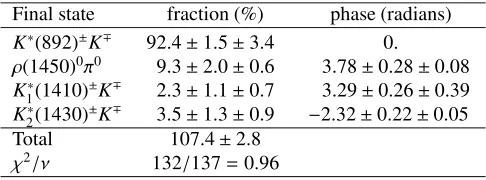
Table 3.Results from the Dalitz-plot analysis of theJ/ψ → K+_K−_π0_{signal region. When two uncertainties are}

given, the first is statistical and the second systematic.

Final state fraction (%) phase (radians) K∗(892)±_K∓ _{92.4±1.5±3.4 0.}

ρ(1450)0_π0 _{9.3±2.0±0.6 3.78±0.28±0.08} K∗

1(1410)

±_K∓ _{2.3±1.1±0.7 3.29±0.26±0.39}

K∗

2(1430)

±_K∓ _{3.5±1.3±0.9 −2.32±0.22±0.05} Total 107.4±2.8

χ2/ν 132/137=0.96

Table 4.Results from the Dalitz-plot analysis of theJ/ψ → K0

SK

±_π∓_{signal region. When two uncertainties are}

given, the first is statistical and the second systematic.

Final state fraction (%) phase (radians) K∗_{(892) ¯K 90.5±0.9±3.8 0.}

ρ(1450)±_π∓ _{6.3±0.8±0.6 −3.25±0.13±0.21}

K∗

1(1410) ¯K 1.5±0.5±0.9 1.42±0.31±0.35 K∗

2(1430) ¯K 7.1±1.3±1.2 −2.54±0.12±0.12 Total 105.3±3.1

χ2_{/ν 274/217=1.26}

7 Ackowledgements

This work was supported (in part) by the U.S. Department of Energy, Office of Science, Office of Nuclear Physics under contract DE-AC05-06OR23177.

References

[1] J. P. Leeset al.[BaBar Collaboration], Phys. Rev. D89, no. 11, 112004 (2014) [2] Charge conjugation is implied through all this work.

[3] S. Eidelmanet al.[Particle Data Group], Phys. Lett. B592, no. 1-4, 1 (2004).

[4] E. M. Aitalaet al.[E791 Collaboration], Phys. Rev. D73, 032004 (2006) Erratum: [Phys. Rev. D 74, 059901 (2006)]

[5] D. Astonet al., Nucl. Phys. B296, 493 (1988). [6] K. M. Watson, Phys. Rev.88, 1163 (1952).

[7] L. Chenet al.[MARK-III Collaboration], SLAC-PUB-5674.

[8] M. Ablikimet al., (BESIII Collaboration), Phys. Lett. B710, 594 (2012). [9] M.E.B. Franklinet al., (Mark II Collaboration) Phys. Rev. Lett.51, 963 (1983). [10] F. Vannucciet al., (Mark I Collaboration) Phys. Rev. D151814 (1977). [11] C. Zemach, Phys. Rev.133, B1201 (1964).

[12] C. Dionisiet al., Nucl. Phys. B169, 1 (1980).