312 | P a g e
A SURVEY: PRINCIPAL COMPONENT ANALYSIS (PCA)
Sumanta Saha
1, Sharmistha Bhattacharya (Halder)
2 1Department of IT, Tripura University, Agartala,(India)
2
Department of Mathematics, Tripura University, Agartala, (India)
ABSTRACT
Principal component analysis (PCA) is one of the most widely used multivariate techniques in statistics. It is
commonly used to reduce the dimensionality of data in order to examine its underlying structure and the
covariance/correlation structure of a set of variables. It is a statistical procedure that uses an orthogonal
transformation to convert a set of observations of possibly correlated variables into a set of values of linearly
uncorrelated variables called principal components. The number of principal components is less than or equal
to the number of original variables. It is a way of identifying patterns in data, and expressing the data in such a
way as to highlight their similarities and differences. This is the survey paper of the existing theory and
techniques for PCA with example.
Keywords:
Correlation structure, Covariance structure,
Multivariate Technique, Orthogonal
Transformation, Principal Component.
I. INTRODUCTION OF PRINCIPAL COMPONENTS ANALYSIS (PCA)
Principal component analysis (PCA) is a statistical procedure that uses orthogonal transformation to convert a
set of observations of possibly correlated variables into a set of values of linearly uncorrelated variables are
called principal components. The number of principal components are less than or equal to the number of
original variables. This transformation is defined in such a way that the first principal component has the largest
possible variance (that is, accounts for as much of the variability in the data as possible), and each succeeding
component in turn has the highest variance possible under the constraint that it be orthogonal to (i.e.,
uncorrelated with) the preceding components [3]. Principal components are guaranteed to be independent if the
data set is jointly normally distributed. PCA is sensitive to the relative scaling of the original variables.
Many papers of PCA are survey here and find that, no papers are combined with the techniques of PCA and the
relevant example. That’s why this type of paper is written where all these things are combined together which is
easy to understand the beginner.
PCA is a widely used mathematical tool for high dimension data analysis. Just within the fields of computer
graphics and visualization alone, PCA has been used for face recognition [10], motion analysis and synthesis
[7], clustering [4], dimension reduction [2], etc.
II. A BRIEF HISTORY OF PRINCIPAL COMPONENTS ANALYSIS
PCA was invented in 1901 by Karl Pearson [6], as an analogue of the principal axis theorem in mechanics; it
was later independently developed (and named) by Harold Hotelling in the 1930s[1]. Depending on the field of
313 | P a g e
Hotelling transform in multivariate quality control, proper orthogonal decomposition (POD) in mechanical
engineering, singular value decomposition (SVD) of X (Golub and Van Loan, 1983), eigenvalue decomposition
(EVD) of XTX in linear algebra, factor analysis, Eckart–Young theorem (Harman, 1960), or Schmidt–Mirsky
theorem in psychometrics, empirical orthogonal functions (EOF) in meteorological science, empirical eigen
function decomposition (Sirovich, 1987), empirical component analysis (Lorenz, 1956), quasiharmonic modes
(Brooks et al., 1988), spectral decomposition in noise and vibration, and empirical modal analysis in structural
dynamics.
III. PCA TECHNIQUES
The techniques of PCA are collected from [5] where a 2-D facial image can be represented as 1-D vector by
concatenating each row (or column) into a long thin vector. Let’s suppose we have M vectors of size N (= rows
of image ×columns of image) representing a set of sampled images. pj’s represent the pixel values:
The images are mean centered by subtracting the mean image from each image vector. Let m represent the mean
of that image:
And let wi be defined as mean centered image:
The main goal is to find a set of ei’s which have the largest possible projection onto each
of the wi’s and to find a set of M orthonormal vectors ei for which the quantity:
is maximized with the orthonormality constraint.
It has been shown that the ei’s and i’s are given by the eigenvectors and eigenvalues of the covariance matrix:
where W is a matrix composed of the column vectors wi placed side by side. The size of C is N × N which could
be enormous. For example, images of size 64 × 64 create the covariance matrix of size 4096 × 4096. It is not
314 | P a g e
ei and scalars i can be obtained by solving for the eigenvectors and eigenvalues of the M × M matrix W
T
W. Let
diand i be the eigenvectors and eigenvalues of WTW, respectively.
By multiplying left to both sides by W:
which means that the first M-1 eigenvectors eiand eigenvalues i of WW
T
are given by Wdiand i, respectively.
Wdi needs to be normalized in order to be equal to ei. Since we only sum up a finite number of image vectors, M,
the rank of the covariance matrix cannot exceed M-1 (The -1 come from the subtraction of the mean vector m).
The eigenvectors corresponding to nonzero eigenvalues of the covariance matrix produce an orthonormal basis
for the subspace within which most image data can be represented with a small amount of error. The
eigenvectors are sorted from high to low according to their corresponding eigenvalues. The eigenvector
associated with the largest eigenvalue is one that reflects the greatest variance in the image. That is, the smallest
eigenvalue is associated with the eigenvector that finds the least variance. They decrease in exponential fashion,
meaning that the roughly 90% of the total variance is contained in the first 5% to 10% of the dimensions.
A facial image can be projected onto M (<< M) dimensions by computing
where vi = eTi wi, vi is the ith coordinate of the facial image in the new space, which come to be the principal
component. The vectors ei are also images, so called, eigen images, or eigenfaces. They can be viewed as
images and indeed look like faces. So, describes the contribution of each eigenface in representing the facial
image by treating the eigen faces as a basis set for facial images. The simplest method for determining which
face class provides the best description of an input facial image is to find the face class k that minimizes the
Euclidean distance
Where k is a vector describing the kth face class. If k is less than some predefined threshold , a face is
classified as belonging to the class k
.
IV. EXAMPLE OF PCA
The example of PCA are collected from [9] and the steps are:
Step 1: Get some data
For this example self-created data set is used. It is the 2 dimension data set, which provide the plots of data to
show PCA analysis at each step.
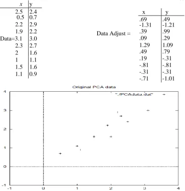
The data is given in Figure 4.1, along with a plot of that data.
Step 2: Subtract the mean
For PCA to work properly, subtract the mean from each of the data dimensions. The mean subtracted is the
average across each dimension. So, all the x values have x (the mean of the x values of all the data points)
315 | P a g e
Data Adjust =
Figure 4.1: PCA example data, original data on the left, data with the means subtracted on the right, and
a plot of the data.
Step 3: Calculate the covariance matrix
Covariance is always measured between 2 dimensions. If a data set having more than 2 dimensions, there is
more than one covariance measurement that can be calculated. Since the data is 2 dimensional, the covariance
matrix will be 2 x 2. The result is given below:
So, since the non-diagonal elements in this covariance matrix are positive, then both the x and y variable may be
increased together.
Step 4: Calculate the eigenvectors and eigenvalues of the covariance matrix
Since the covariance matrix is square, then calculate the eigenvectors and eigenvalues for this matrix. In the
meantime, here the eigenvectors and eigenvalues are:
x
y
2.5 2.4
0.5 0.7
2.2 2.9
1.9 2.2
Data=3.1
3.1
3.0
2.3 2.7
2
1.6
1
1.1
1.5 1.6
1.1 0.9
x
y
.69
.49
-1.31
-1.21
.39
.99
.09
.29
1.29
1.09
.49
.79
.19
-.31
-.81
-.81
-.31
-.31
316 | P a g e
It is important to notice that these eigenvectors are both unit eigenvectors i.e. their lengths are both 1. This is
very important for PCA, but luckily, most math packages, when asked for eigenvectors, will give unit
eigenvectors.
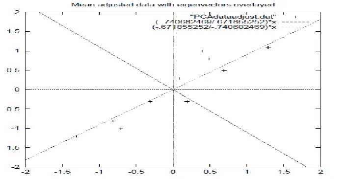
If look at the plot of the data in Figure 4.2 then see how the data has quite a strong pattern. As expected from the
covariance matrix, two variables increase together. They appear as diagonal dotted lines on the plot. As stated in
the eigenvector section, they are perpendicular to each other. But, more importantly, they provide us with
information about the patterns in the data. So, by this process of taking the eigenvectors of the covariance
matrix, now extract lines that characterize the data. The rest of the steps involve transforming the data so that it
is expressed in terms of them lines.
Step 5: Choosing components and forming a feature vector
Here is where the notion of data compression and reduced dimensionality comes into it. If look at the
eigenvectors and eigenvalues from the previous section, notice that the eigenvalues are quite different values. In
fact, it turns out that the eigenvector with the highest eigenvalue is the principle component of the data set.
Figure 4.2: A plot of the normalized data (mean subtracted) with the eigenvectors of the covariance
matrix overlayed on top.
In this example, the eigenvector with the larges eigenvalue was the one that pointed down the middle of the
data. It is the most significant relationship between the data dimensions.
In general, once eigenvectors are found from the covariance matrix, the next step is to order them by eigenvalue,
highest to lowest. This gives the components in order of significance. Now, if user like, user can decide to
ignore the components of lesser significance. Then user loses some information, but if the eigenvalues are small,
317 | P a g e
original. To be precise, if originally have n dimensions in data set, and want calculate n eigenvectors and
eigenvalues, and then choose only the first p eigenvectors, then the final data set has only p dimensions.
Now need a feature vector, which is just a fancy name for a matrix of vectors. This is constructed by taking the
eigenvectors that are kept store in the form of eigenvectors, and forming a matrix with these eigenvectors in the
columns.
Feature Vector = (eig1 eig2 eig3.... eign)
In this example 2 eigenvectors are found and have the two choices either form a feature vector with both of the
eigenvectors:
or, can choose to leave out the smaller, less significant component and only have a single column:
Finally the result of each of these eigenvectors is found in the next section.
Step 6: Deriving the new data set
This is the final and easiest step of PCA. Once the chosen components (eigenvectors) can be kept in data set and
formed a feature vector, then simply take the transpose of the vector and multiply it on the left of the original
data set, transposed.
Final Data = Row Feature Vector × Row Data Adjust,
where Row Feature Vector is the matrix with the eigenvectors in the columns transposed so that the
eigenvectors are now in the rows, with the most significant eigenvector at the top, and Row Data Adjust is the
mean-adjusted data transposed, i.e. the data items are in each column, with each row holding a separate
dimension. Final Data is the final data set, with data items in columns, and dimensions along rows. It will give
the original data solely in terms of the vectors has been chosen. The original data set had two axes, x and y, so
the data was in terms of them. It is possible to express data in terms of any two axes. If these axes are
perpendicular, then the expression is the most efficient. This was why it was important that eigenvectors are
always perpendicular to each other. The data is being changed in terms of the axes x and y, and now they are in
terms of 2 eigenvectors. In this case the new data set has reduced dimensionality.
To show this data and doing the final transformation with each of the possible feature vectors. Taking the
transpose of the result in each case to bring the data back to the nice table like format and also plotted the final
points to show how they relate to the components.
In the case of keeping both eigenvectors for the transformation, now get the data and the plot found in Figure
4.2. This plot is basically the original data, rotated so that the eigenvectors are the axes. This is understandable
since we have lost no information in this decomposition.
The other transformation that can make is by taking only the eigenvector with the largest eigenvalue. The table
of data resulting from that is found in Figure 4.1. As expected, it only has a single dimension. If compare this
318 | P a g e
column of the other. So, if plot this data, it would be 1 dimensional, and would be points on a line in exactly the
x positions of the points in the plot in Figure 4.3.
Getting the old data back
Wanting to get the original data back is obviously of great concern, if the PCA transform for data compression
is used.
Transformed Data=
Data transformed with 2 eigenvectors
Figure 4.3: The table of data by applying the PCA analysis using both eigenvectors, and a plot of the new
data points.
X
Y
-.87970186
-.175115307
1.77758033
.142974
-.992197494
.310374989
-.274210416
.130417207
-1.67580142
-.209491061
-.912949103
.17521044
.0991094375
-.34910698
1.14457216
.046417258
.438046137
.0177646297
319 | P a g e
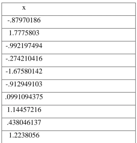
Transformed Data (Single eigenvector)
x
-.87970186
1.7775803
-.992197494
-.274210416
-1.67580142
-.912949103
.0991094375
1.14457216
.438046137
1.2238056
Figure 4.4: The data after transforming using only the most significant eigenvector
So, how do get the original data back? Before do that, remember that only if to took all the eigenvectors in our
transformation will get exactly the original data back. If the number of eigenvectors are reduced in the final
transformation, then the retrieved data has lost some information. Recall that the final transform is this:
Final Data = RowFeatureVector × Row Data Adjust,
which can be turned around so that, to get the original data back,
RowDataAdjust = RowFeatureVector-1× Final Data
where RowFeatureVector~1is the inverse of RowFeatureVector. However, when take all the eigenvectors in our
feature vector, it turns out that the inverse of our feature vector is actually equal to the transpose of our feature
vector. This is only true because the elements of the matrix are all the unit eigenvectors of our data set. This
makes the return trip to our data easier, because the equation becomes
RowDataAdjust = RowFeatureVectorT× Final Data
But, to get the actual original data back, need to add on the mean of that original data (remember we subtracted
it right at the start). So, for completeness,
RowOriginalData = (RowFeatureVectorT× Final Data) + Original Mean
This formula also applies to when you do not have all the eigenvectors in the feature vector. So even when you
leave out some eigenvectors, the above equation still makes the correct transform.
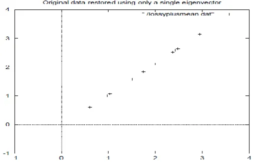
However, I will do it with the reduced feature vector to show you how information has been lost. Figure 4.5
320 | P a g e
Figure 4.5: The reconstruction from the data that was derived using only a single eigenvector
Compare it to the original data plot in Figure 4.1 and you will notice how, while the variation along the principle
eigenvector (see Figure 4.2 for the eigenvector overlayed on top of the mean-adjusted data) has been kept, the
variation along the other component (the other eigenvector that we left out) has gone.
V. CONCLUSION
Principal Component Analysis is powerful statistical techniques. PCA is used to find optimal ways combining
variables into a small number of subsets. Principal Component Analysis are useful as data reduction but not for
understanding the structure of the data. This paper deals with the history of PCA and the ideas of PCA. It also
discusses the technique of PCA with example.
REFERENCES
[1] H. Hotelling, (1933). Analysis of a complex of statistical variables into principal components. Journal of
Educational Psychology, 24, 417–441, and 498–520.
[2] S. Huang, M. O. Ward, and E. A. Rundensteiner. Exploration of dimensionality reduction for text
visualization. In CMV '05: Proceedings of the Coordinated and Multiple Views in Exploratory Visualization,
pages 63-74, Washington, DC, USA, 2005. IEEE Computer Society.
[3] I. T. Jollie, Principal Component Analysis. Springer, second edition, 2002.
[4] Y. Koren and L. Carmel. Visualization of labeled data using linear transformations. InfoVis, 00:16, 2003.
[5] Kyungnam Kim, Face Recognition using Principle Component Analysis.
[6] K. Pearson, (1901). On Lines and Planes of Closest Fit to Systems of Points in Space (PDF). Philosophical
Magazine 2 (11): 559–572. doi:10.1080/14786440109462720.
[7] A. Safonova, J. K. Hodgins, and N. S. Pollard. Synthesizing physically realistic human motion in
low-dimensional, behavior-specic spaces. ACM Trans.Graph., 23(3):514-521, 2004.
[8] Jon Shlens, A tutorial on Principal Component Analysis, 25 March,2003.
[9] Lindsay I Smith, A tutorial on Principal Component Analysis, February 26, 2002.
[10] M.A. Turk and A.P. Pentland, Face Recognition Using Eigenfaces, IEEE Conf. on Computer Vision and