AN ENERGY AWARE RESOURCE ALLOCATION MODEL FOR CLOUD COMPUTING

AN ENERGY AWARE RESOURCE ALLOCATION

MODEL FOR CLOUD COMPUTING

Shahadat Hussain



Zahid Raza

1,2

School of Computer and Systems Sciences, Jawaharlal Nehru University, New Delhi, (India)

ABSTRACT

Cloud computing is a model for enabling ubiquitous, convenient, on-demand access to a shared pool of

resources which offer subscription-oriented IT services like compute, apps, data, etc, as a service. The

end-users simply makes utilization of the services available over the cloud infrastructure and pay in support of the

used services. Various criteria determine the quality and production cost of the service. The duration of this

service (makespan) and the consumed energy are two such important criteria. Most of the works reported in the

literature propose algorithms to minimize the completion time (makespan) with less focus on energy

consumption. This work proposes a scheduling model with an algorithm takes into account even energy

consumption along with makespan of the task submitted as DAG. The algorithm first considers the variation of

energy consumption of processors then selects the job module based on the highest upward rank and schedules

it to the processor which dissipates minimum computational energy in an insertion-based approach.

Keywords

:

Cloud Computing, Directed Acyclic Graph, Heterogeneous Computing System,

Precedence Based Scheduling, Rank of Job Modules, Minimized Energy Consumption, and

Makespan.

I. INTRODUCTION

II. THE PROPOSED MODEL

The model under consideration is a task scheduling strategy which supports execution of computationally intensive

dependent modules over a diverse set of interconnected processors. The algorithm takes two inputs viz. a computationally intensive job and returns schedule with turnaround time with energy consumption as output. The terms task and module are interchangeably used in the upcoming sections.

2.1 Job Characteristics

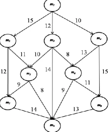
A job is assume to be in the form of directed acyclic graph (DAG)G =(V, E), where V is set of v nodes and E is a set of e directed edges. A node in the DAG corresponds to a module (m1, m2, m3, …,mn) which a set of

instructions that must be executed sequentially without preemption over a single processor. The weight of a module mi over processor Pj is denoted by wij. Modules can be independent or dependent from other modules of

the same job. Independent modules can be executed without any delay but dependent modules have to wait for their parents to initialize their execution. The communication cost between two modules assigned to the same processor is assumed to be zero while over different processor it is non zero. Module m1and mn are termed as

entry and exit modules respectively. A sample job with the above considerations is presented in Fig. 1.

Fig. 1: A Sample Job Representation by Directed Acyclic Graph (DAG).

2.2 Heterogeneous Computing System

The proposed algorithm assumes the target computing environment is a set p of interconnected heterogeneous processors and is represented by p = {px : 1 ≤ x ≤ N }. Each processor px is represented by a vector (fx, vx, cx)

where fx, vx and cx represents the operating frequency, voltage required to sustain the frequency and capacitance

of the processor px. Each processor is composed of a local memory unit and do not share memory of other

operating in two states, either they are processing a job module or sitting idle. Section 2.6 presents power consumption model by the processors.

2.3

The Scheduler

When a job is submitted to the scheduler it creates a list of modules from the given task graph according to their priorities in non increasing order. Following that it selects the ready module with highest priority from the list and assigns it to the suitable processor that minimizes the processing energy of the module. The algorithm under study is recursive and static [8] as the scheduler has all the information about task precedence, parallelism in modules and architecture of processors inter-connectivity a priory.

2.4 Parameters Used

In order to achieve efficient schedule of a job G on heterogeneous processors, it is required to define the following basic parameters:

 Processor Ready Time (RTi ): It is the time duration for which processor pi is available for execution.

 Earliest Start Time (ESTi ):It is defined as starting time of module mi over the processor where it can be

started as early as possible and can be written as:

E , If the number of immediate parents are zero.

If number of parents are k (1)

Where k (> 0) represents number of immediate parents [9].

 Earliest Finish Time (EFTi): Earliest finish time of the scheduled module mi over the processor pj is

defined as the sum ofEST and Computation Time Wijof the module. It can be written as [9] :

(2)

 Turnaround Time (TATj): It is defined as the total time taken between the submission of the job for

execution and return of the completion output to the user which is calculated as [7, 9] :

(3)

2.5 Prioritization of Job Modules

Before scheduling, each module mi is labeled with the average computation cost which is defined as:

(4)

For the exit module mexit the upward rank value is equal to:

(5) The upward rank of a module (mi ) other than exit modules is recursively defined as [9]:

(6)

Where is the average communication cost of edge (i, j).

Modules are sorted in non decreasing order based on their ranku value. Tie-breaking is done randomly. The non

increasing order of ranku values presents a topological order of modules which is a linear order that preserves

2.6

Energy Consumption Model

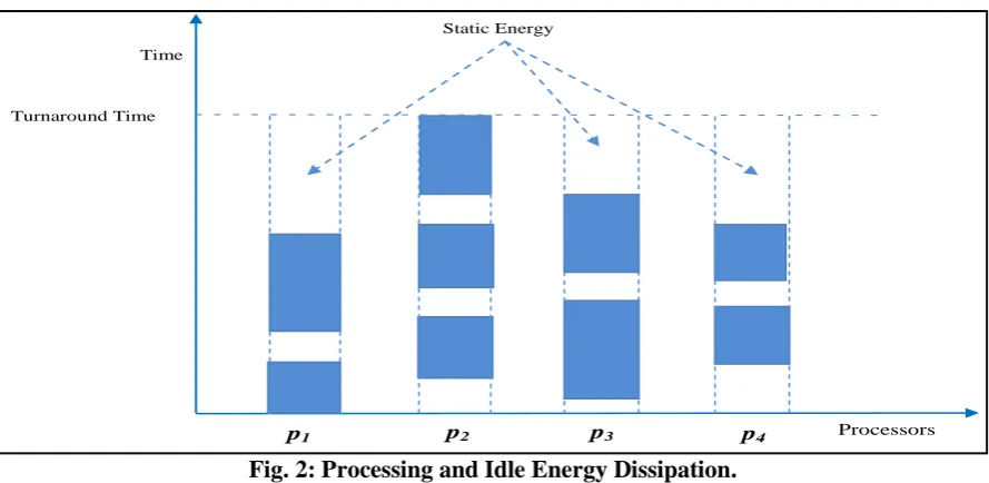
The energy consumed by processor while executing a job denoted by Etotal is composed of static energy Estatic

that is energy dissipated while processor is sitting idle and processing energy Eprocessing which is the amount of

energy consumed when the processor is specifically processing the job modules. A typical scenario of consumption of processing energy and static idle energy has been presented in fig. 2.

Fig. 2: Processing and Idle Energy Dissipation.

The power dissipated while processing a job module ρprocessing with a CMOS (Complementary Metal Oxide

Semiconductor) based microprocessor is computed as:

(7) Thus, the energy consumed by a processor pi while processing module mkis computed as:

(8) where Wikis the computation cost of module mion the processor pk [7, 10].

In the job execution period, we assume that the processorsoperate at the highest level of supply voltage and at highest frequency. However they scale down their voltage and frequency to lowest supply voltage and lowest operational frequency during idle period. The total energy consumed by a processor while sitting idle Estatic can

be computed as:

(9) Where ti and are the idle time and power dissipation respectively of processor pi while sitting idle [7,

10].

The total energy consumed during processing the job module is computed as:

(10)

Where (RTi - ti) is the total time during which processor pi was executing the job modules with the utilization

of power of processor. Therefore, the total of computation for the entire job is given as [7, 10]:

(11)

Static Energy

Turnaround Time Time

p2 p3 p4 Processors

2.7 Proposed Algorithm

The scheduler works according to the following mechanism which is described below in the following steps.

Alloc Energy

alloc_energy ( )

{

Evaluate the mean value of computation cost of all the job modules Construct a list of modules in reversed topological order i.e. RevTopoList

{

for each module mi in RevTopoList do

if module is exit module ranku of exit module =

endif

max = 0

for each child my of module mi do

if Ciy + ranku (my) > max then max = Ciy + ranku (my)

endif endfor

ranku (mi) = + max

endfor }

Sort the modules of scheduling list in non increasing order of their ranku value

{

while there is unscheduled module in the list do

Select the first module mi from the list for scheduling

for each processor pkin the processor- set (pk p) do

Calculate expected computation energy matrix ECE (mi, pk)

Assign module mito the processor pk that has minimum value in the ECE

matrix for module mi

endfor endwhile }

Turnaround time of the job is calculated as per equation (3) {

for each processor px p

}

Total energy for the entire job is calculated as sum of static and processing energy using equation (11)

}

In the first step modules of the entire job are leveled with average computation cost which is calculated based on the equation (4) and list of modules in the reverse topological order are generated.

In second step ranku value for all modules are evaluated by taking in account the mean computation cost of

module and communication cost from each child of the module. The detailed description for the upward rank evaluation has been provided in section 2.5.

In third step the modules are sorted with their rank value in non increasing order and a list is generated.

Following step starts with first modules mi in the list. The algorithm searches for an appropriate idle time slot

for module mi onto the processor pj which results in offering minimum computational energy, at the time when

all input data of mi sent by mi„s immediate predecessors modules have arrived at processor pj. The search

extended until finding of first idle time slots which is capable of holding the computational cost of module mi.

The module is removed from the list and the process is repeated until all the modules in the list get scheduled. The expected computational energy of modules for all processors is evaluated using equation (10) and is provided in ECE matrix.

Later when all modules get allocated on to the processors, turnaround time is evaluated and presented as one of the outputs of the algorithm which is equal to entire time taken from the submission of the job to the earliest finish time of exit module.

In the last step static and processing energy for all the processors are computed seperately by using equations (9) and (10). Total computational energy for entire job computed as summation of all static and processing energy dissipated using equation (11) and presented as output of the algorithm.

III. ILLUSTRATIVE EXAMPLE

In order to get better understand the model, an illustrative example for a typical job is presented here. The parameters have been scaled down for illustration purpose only; however the model is capable to work with any data values. The illustration considers a scenario where four heterogeneous processors are fully interconnected and are available for execution. The schedule for every module allocated on a processor can be characterized as pn [ESTi, mi, EFTi] with EST and EFT values of the module. In the beginning, all processors are assumed to be

idle. Since the job bounded for computation is represented in the form of DAG, let us assume the job presented in Fig. 1 as a sample job for execution. The job comprises of nine modules m1, m2, m3… m9 that are represented

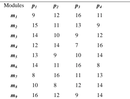
by a circle having an entry for module number. The edges linking different modules correspond to the Communication Cost (Cij) between modules. The expected computation cost matrix (ECC) for the job is given

in the Table 1 of which each entry ECC(i,j) denotes expected computation cost of module mi over processor pj

Table 1 Expected Computation Cost Matrix

Modules p1 p2 p3 p4

m1 9 12 16 11

m2 15 11 13 9

m3 14 10 9 12

m4 12 14 7 16

m5 13 9 10 14

m6 14 11 16 8

m7 8 16 11 13

m8 10 8 12 14

m9 16 12 9 14

As per described in algorithm in section 2.7, we first evaluate the mean value of the expected computation cost for each module by the help of equation (4). Modules with their value are listed in the Table 2.

Table 2 Modules with their

Modules

m1 12.00

m2 12.00

m3 11.25

m4 12.25

m5 11.50

m6 12.25

m7 12.00

m8 11.00

m9 12.75

With the utilization of and Cij values in equation (5) and (6) the upward rank values for each module

calculated and is presented as Table 3.

Table 3 Upward Rank of the Job Modules

Modules ranku

m1 109.25

m2 82.25

m3 80.50

m4 85.25

m5 59.25

m6 60.00

m7 38.75

m8 36.75

After the calculation of ranku values, priorities are assigned to each module. The highest priority is given to the

module which has highest value for ranku. The modules are ordered as per their ranku value in non increasing

order. Hence, the final priority list of modules is presented as

m1 m4 m2 m3 m6 m5 m7 m8 m9

Let us assume there are four heterogeneous hypothetical processors that are fully interconnected and all inter processor communications between them are assumed to be performed without contention. The proposed algorithms assume computation and communications are overlapped with each other. Since processors are under consideration are available with two state of operation the power dissipated by them differs accordingly. Depends on their state of operations, typical parameters of four processors under consideration are described in Table 4

Table 4 Parameters of Heterogeneous Processors

Processors _c(10-10 _Farad)

v

p1 65.2 254 1.44 2.58 135.88

p2 37.2 278 1.30 2.28 107.11

p3 50.0 266 1.52 2.64 162.24

p4 77.0 292 1.36 2.32 125.30

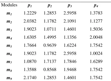
The algorithm considers the power dissipated by processors while sittinlg idle is that is fixed and the corresponding value for each processor is given in the Table 4. The power dissipated by the processors during the execution of job modules is termed as and is calculated by the use of equation (7). The Expected Computational Energy Matrix ECE[n][p] has been presented in Table 5 as given below:

Table 5 Expected Computational Energy Matrix

Modules p1 p2 p3 p4

m1 1.2229 1.2853 2.5958 1.3783

m2 2.0382 1.1782 2.1091 1.1277

m3 1.9023 1.0711 1.4601 1.5036

m4 1.6305 1.4995 1.1356 2.0048

m5 1.7664 0.9639 1.6224 1.7542

m6 1.9023 1.1782 2.5958 1.0024

m7 1.0870 1.7137 1.7846 1.6289

m8 1.3588 0.8568 1.9468 1.7542

m9 2.1740 1.2853 1.4601 1.7542

The search for an appropriate idle time slot of a module mi on a processor pj starts at time equal to ESTi of mi on

Fig. 3: Schedule for the Job Considered In Illustrative Example

That means the time when all input data of mi sent by mi‟s immediate predecessor modules have arrived on

processor pj. The search continues until finding the first idle time slot that is capable of holding the computation

cost of module mi. Entries ECE(i, j) of matrix represents the energy consumed by processors while executing

the module the value of which are provided by calculation based on equation (8). The final schedule for job considered in our example is generated according to the entries in Table 5. and is presented in fig 3.

After all the modules of the job is scheduled the turnaround time of the job is calculated using the equation (3). In this algorithm the turnaround time of job is simply EFT (Earliest Finish Time) of the exit module mexit.

Therefore the turnaround time for the entire job is given as:

TATj = 96.00 milliseconds.

The idle time and processing time for each processor during the job execution are summarized as:

Processors p1 p2 p3 p4

Idle Time ( ti ) 79 57 89 79

Processing Time (TAT-ti) 17 39 7 17

The total energy consumption Etotal accounts for both the energy required to execute the assigned modules, and

the energy that each processor consumes while sitting idle which is calculated by th help of equations (9), (10) and( 11). The split of static and processing energy by each processor are shown in tabular form given below as:

Processors p1 p2 p3 p4

Static Energy (Joule) 5.151 2.12 4.45 6.08 Processing Energy (Joule) 2.30 4.17 1.13 2.13

The summation of static energy dissipated by all the processors while executing the job is found to be:

Estatiic = 17.8042 Joule.

Similarly, the energy consumed by all the processors while processong the job is calculated which is equal to:

Eprocessing = 09.7527 Joule.

The total energy dissipated while execution of the entire job is summation of static and processing energy consumed by the processors which is equal to:

IV. SIMULATION RESULTS

To evaluate the performance of the proposed model in terms of energy consumption and schedule length rigorous simulation runs were conducted. Simulation runs were carried out on Intel Core i7-3770, 3.4 GHz, 6.0 GB RAM machine running under Windows 7 Professional 64-bit Operating System. The programming language of choice was MATLAB R2013a (Version 8.1). While observing total computational energy (Etotal)

and turnaround time for the job (TATj) the model was simulated with different consideration taking into

account for example running a job with different number of modules over fixed number of processors and running a single job over different number of processors. The same job is then simulated using the scheduling strategy of round-robin and the Etotal observed is then compared with the Etotal obtained with the proposed

model. The results are summarized as Fig. 4. It can be observed that the scheduling strategy based on proposed algorithm always results in less Etotal.

Fig. 4 Analysis of Computational Energy Consumptions

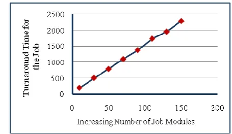
For the above experiments, the TATj generated for each job has also been determined and plotted against

increase in the job modules as shown in Fig. 5

Fig. 5 Turnaround Time of Job Modules with Increase in Numbers of Modules in Job.

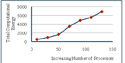
The next set of experiments intended to observe the effect of the change in Etotal for the same job with varying

Fig. 6: Variation of Computational Energy with Increase in Number of Processors.

V. OBSERVATIONS

 The allocation of modules gets affected by the two factors considered for allocation viz. computational energy of module on to a processor, time to finish execution of the previous workload on to a processor.

 The proposed model allocates modules on to the processor which consume minimum computational energy among all while taking care the dependency of module.

 For a fixed number of processors, total computational energy increases with increase in modules of the job as processors have to execute large number of modules.

 Processors may have two working states i.e. idle and processing states. The energy consumption rate is different under different modes.

 The total computational energy increases with the increase in number of processors for the same job becouse idle time of processors increases hence static energy.

 Execution of a job on the distributed systems incurs a substantial communication cost which results in

increase in turnaround time with increase in number of modules in the job.

Many experiments were conducted to study the behavior of the model but the results obtained were observed to be along the same line as reported in this work.

REFERENCES

[1]. Buyya, R., Shin Yeo, C., Venugopal, S., Broberg, J., & Brandic, I. (2009). Cloud computing and emerging IT platforms: Vision, hype, and reality for delivering computing as the 5th utility. Future Generation Computer Systems, 25(6), 599–616., ISSN 0167-739X.

[2]. Ullman JD (1975) “NP-complete scheduling problems.” J Comput Syst Sci 10(3):384–393.

[3]. Raza Abbas Haidri,C. P. Katti, P. C. Saxena,A Load Balancing Strategy for Cloud Computing Environment, IEEE conference,2014, 636-641.

[4]. Shahid M, Raza Z. “Level based batch scheduling strategy with idle slot reduction under DAG constraints for computational grid”, Journal of Systems and Software, Elsevier, Volume 108, October 2015, Pages 110–133.

[6]. J. Mei, K. Li, K. Li, “Energy-aware task scheduling in heterogeneous computing environments”, Cluster Computing, 17 (2), pp. 537–550, 2012.

[7]. Yu-Kwong Kwok, Ishfaq Ahmad, “Static Scheduling Algorithms for Allocating Directed Task Graphs to Multiprocessors,” ACM Computing Surveys (CSUR), v.31 n.4, p.406-471, Dec. 1999.

[8]. Topcuoglu H, Hariri S, Wu M-Y. ”Performance-Effective and Low-Complexity Task Scheduling for Heterogeneous Computing”. IEEE Transactions on Parallel and Distributed Systems, 13(3), pp.260–274, 2002.

[9]. C. Lee and A. Zomaya, and ldquo, “Energy Conscious Scheduling for Distributed Computing Systems under Different Operating Conditions”, IEEE Trans. Parallel and Distributed Systems, vol. 22, no. 8, pp. 1374-1381, Aug. 2011.