Flexibly Nested Production Functions: Implementation for MONASH

Eleventh Floor Menzies Building

PO Box 11E, Monash University Wellington Road

CLAYTON Vic 3800 AUSTRALIA

Telephone: from overseas:

(03) 9905 2398, (03) 9905 5112 61 3 9905 5112 or 61 3 9905 2398

Fax:

(03) 9905 2426 61 3 9905 2426

e-mail [email protected]

web site http://www.monash.edu.au/policy/

F

LEXIBLY

N

ESTED

P

RODUCTION

F

UNCTIONS

:

Implementation for M

ONASH

by

R. A. McDougall

Centre of Policy Studies

Monash

University

Preliminary Working Paper No. IP–57 June 1992

reissued October 2001

C

ENTRE

of

P

OLICY

S

TUDIES

and

the

I

MPACT

ABSTRACT

This paper describes the implementation for the MONASH model of a scheme for flexible nesting of production functions. The scheme supports substitution in production between different commodities and between commodities and primary factors, which the standard ORANI production system does not. Thus it supports more flexible functional forms than standard ORANI.

More importantly, this treatment supports not just a single functional form but a wide variety of functional forms, built up by the nesting of CES aggregator functions. The number of CES aggregator functions, their membership, and the depth of nesting are all arbitrary. These features of the nesting structure are now specified not in the theoretical structure in the database. Thus the production structure can readily be modified to meet the special requirements of individual applications.

Contents

Abstract i

1. Design 2

2. Theoretical structure 5

3. Implementation 11

4. Illustrative application 16

References 18

Appendix 1: Additions to the TABLO source code for the flexibile

Nesting treatment 19

Appendix 2: Energy sectors in a version of ORANI-E 26 Appendix 3: Data added to an ORANI-E database to model

inter-fuel and energy-capital substitution with

the flexible nesting treatment 27

Tables and Figures

Table 1: Production-related variables with flexible nesting:

Mnemonics and treatment in condensation 13

Table 2: Arrays added to the invariant parameters file for the

flexible nesting treatment 14

Figure 1: Standard production structure in ORANI 4

FLEXIBLY NESTED PRODUCTION FUNCTIONS:

IMPLEMENTATION FOR MONASH

1

by

R.A. McDougall

This paper describes the implementation for the MONASH model of a scheme for flexible nesting of production functions.

MONASH is a multisectoral model of the Australian economy under development at the Centre of Policy Studies (COPS), Monash University (Dixon, Parmenter, Pearson, McDonald, Horridge and Adams 1992). MONASH is a major enhancement and extension of the earlier ORANI model (Dixon, Parmenter, Sutton and Vincent 1982). It will advance beyond ORANI in its treatment of

— dynamics and timeliness of data,

— environment and technology, and

— regions.

Within the area of environment and technology particular attention will be paid to energy use.

Early versions of MONASH inherit from ORANI a production structure in which substitution possibilities are severely restricted. Substitution is not allowed between different intermediate inputs, or between intermediate inputs and primary factors (Dixon et al. 1982, pp. 68-70). For many applications this is unsatisfactory. In energy policy applications for instance inter-fuel and energy-capital substitution effects are often essential to the analysis.

The restrictions on substitution possibilities in ORANI arise both from the nesting of the production function and from the functional form used at the highest level of the nesting structure. At the hightest level a primary factor bundle, individual commodities, and a residual input called ‘other cost tickets’ combine in a fixed-coefficients (Leontief) aggregator function. The Leontief functional form at this level rules out inter-fuel and energy-factor substitution. The separation of

1

The research reported in this paper has been undertaken by the Centre of Policy Studies, as part of the MONASH project and the joint ABARE-CoPS project for system-wide analysis of least cost combinations of options to reduce greenhouse gas emissions. The MONASH project has been undertaken with financial assistance from the Commonwealth Government, through the Industry Commission. The greenhouse gas project has been undertaken with financial assistance from the Commonwealth Department of the Arts, Sport, the Environment, and Territories, and the Victorian Office of the Environment.

energy carriers from primary factors in lower levels rules out any discrimination in energy-factor substitution between capital and other primary factors.

In developing MONASH for energy policy applications the modelling of inter-fuel and energy-capital substitution has a high priority. The obvious approach would be to define a new nesting structure providing for these kinds of substitution explicitly. This new structure however would itself be liable to frequent revision. Revisions would be needed as new information emerged regarding the appropriate nesting of fuels and other energy carriers, new energy carriers were added to the model, or enhancements were made to the treatment of non-energy areas (e.g. substitution between bank and non-bank finance).

A more promising approach is to adopt a flexibly nested production structure. Hanslow (1992) shows how flexibility can be achieved in the membership of nests in the production function, in the number of nests at each level, and even in the number of levels. Changes to the nesting structure do not then require changes to the theoretical structure and source code, but can be made simply by changing nesting information in the database.

We have implemented the flexible nesting treatment in a version of ORANI called ORANI-E, under development for the ABARE-COPS greenhouse gas project. Together with other theoretical and data enhancements in ORANI-E the flexible nesting treatment is intended to be taken over at a later time into MONASH.

This paper describes the implementation of flexibly nested production functions and their application in ORANI-E to energy modelling. Section 1 describes the overall design, and section 2 the detailed changes to the theoretical structure. Sections 3 and 4 describe the implementation and an illustrative application.

1.

Design

We describe nesting structures in terms of fictitious entities called subproducts. Each industry provides subproducts for itself using primary factors, commodities, and (possibly) other subproducts; it uses them either to provide other subproducts or directly to support its overall activity level. The combination of inputs to provide subproducts is described by aggregator

functions; these in effect are production functions for subproducts.

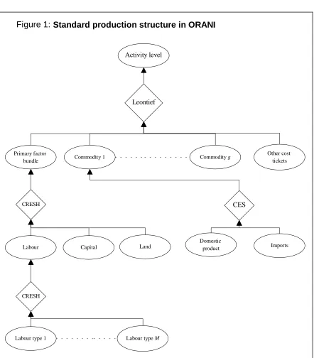
The complete production structure for a typical ORANI industry is depicted in figure 1. At the top of the structure the Leontief function combines the primary factor bundle with ‘effective commodities’ and ‘other cost tickets’ to support industry activity. Effective commodities are constant elasticity of substitution (CES) composites of domestic products and imports (other cost tickets are a residual cost category covering returns to working capital and some indirect taxes). The primary factor bundle as stated above is a CRESH composite of ‘effective labour’, capital, and land. Lastly, effective labour is a CRESH composite of several occupational varieties (Dixon

et al. 1982 pp. 68-74).

In the new treatment we define a theoretical structure which does not specify the nesting structure but reads it from the database. Clearly this new structure is much more flexible than the old. In our initial implementation however we aim not for maximum flexibility but for the minimum consistent with both the standard ORANI production functions and the production structure proposed for the ABARE-COPS greenhouse gas project. Having performed this minimal implementation we can readily provide further flexibility if and when needed.

One way in which the initial implementation is restricted is in scope. It does not cover the bottom level of the nesting structure, where the standard ORANI treatment is left unchanged. This level contains the nest in which the occupational labour varieties combine to form ‘effective labour’, and nests in which the domestically produced and imported varieties of each commodity combine to form ‘effective commodities’. Effective labour and effective commodities are inputs into the flexibly nested part of the structure.

Some change is made at the top of the nesting structure. As in standard ORANI industry activity is provided by a Leontief combination of inputs; but the inputs are now different. They now include some but not necessarily all of the effective commodities, some but not necessarily all subproducts, and other cost tickets. The database specifies which effective commodities and subproducts enter the top nest. Primary factors do not appear in the top level but support activity indirectly as inputs into subproducts.

The greatest changes are made to the middle levels of the nesting structure. Previously this contained just the primary factor nest. Now it contains an arbitrary number of nests describing the composition of subproducts from primary factors, effective commodities, and subproducts. With subproducts entering as inputs into other subproducts, not only the number of nests but also the depth of nesting is arbitrary.

Activity level

Leontief

Primary factor

bundle Commodity 1 Commodity g

Other cost tickets

Capital Land

Domestic

product Imports

CRESH CES

CRESH

Labour type 1 Labour type M

Figure 1: Standard production structure in ORANI

Labour

Another restriction relates to the functional form and parameterisation of the aggregator functions. We impose a CES functional form, with Cobb-Douglas and Leontief available as special cases (standard ORANI uses the more general CRESH form for the primary factor bundle but then sets substitution parameters such that CRESH reduces to CES). We also impose uniformity across industries in elasticities of substitution.

To define the nesting structure we add arrays to the database specifying, for each primary factor, effective commodity, or subproduct, which subproduct it is used to provide. As an alternative to providing subproducts, effective commodities and subproducts but not primary factors may instead enter into the top level of the nesting structure to support industry activity directly. The commodity array has an industry dimension allowing the assignment of commodities to subproducts vary across industries; the primary factor arrays and subproduct arrays have no industry dimension. We provide also an array containing the elasticities of substitution for the CES aggregator functions; this array too lacks an industry dimension, so the elasticity settings do not vary across industries.

2.

Theoretical structure

We adapt notation from Dixon et al. (1982, pp. 68-74). Equations included in the model are displayed in boxes.

In describing a nest we say that a collection of effective commodities, primary factors, and subproducts compose a subproduct, or that the subproduct comprises the collection or the elements of the collection.

As in standard ORANI we have some number g of commodities and three primary factors, but now we have also some number f of subproducts. Also as in standard ORANI we associate with every basic and composite input into production a technology variable. These variables represent input-diminishing technological changes. For each nest in the production function, with all nest inputs but one held fixed, the amount of that input needed for a given nest output is proportional to the corresponding technology variable. The model also contains input-neutral and output-diminishing technological change variables.

We define the nesting structure using various mappings. A function n_F maps primary factors to

subproducts, where for each primary factor v n_F(v) denotes the subproduct comprising v. For

each industry j a function n_C(j) maps effective commodities to subproducts, where for each

effective commodity i n_C(j)(i) denotes the subproduct comprising i. If effective commodity i

enters directly into the top level of the nesting structure we set n_C(j)(i) equal to zero. Likewise a

subproduct comprising v; or if subproduct v appears in the top level of the nesting structure, n_B(v) is equal to zero.

At the top of the production structure is a Leontief production function involving effective commodities and subproducts:

(1) Leontief : ( )( ) 0, ₍₁₎ : ( ) 0 ,

) 1 ( ) 1 ( C ) 1 ( ) 1 (       = =

= n v

A X i j n A X Z

A _j B

Bv j Bv C j i j Ci j

j j = 1,...,h,

where for any set of positive real numbers ;,

Leontief(;) ≡ min(;).

The variables are:

— Z_j, activity in industry j,

— X_Ci( )1j, usage of effective commodity i by industry j,

— X_Bv( )1j, usage of subproduct v by industry j, and

— A( )_j1 , A_Ci( )1j, and A_Bv( )1 j, technology variables.

The middle layer of the production structure contains the subproduction functions:

(2) , , , ; ; ) ( : , ) )( ( : , ) ( :

CES ₍₁₎ (1) (1) (1) (1)

) 1 ( ) 1 ( ) 1 ( ) 1 ( ) 1 ( ) 1 (       = = = = u Bv u Ci u Fv Bu B j Bv j Bv C j Ci j Ci F j Fv j Fv j Bu b b b u v n A X u i j n A X u v n A X X ρ

u = 1,...,f, j = 1,...,h,

where for positive variables X_i, parameter ρ greater than -1 but not equal to zero, and positive

parameters b_i,

{

; ;

}

. CES / 1 ρ ρ ρ − − _      =

∑

i i i i

i b b X

X

The equation contains new variables:

— X_Fv( )1j, employment of primary factor v by industry j, and

— A_Fv( )1 j, a technology variable.

The equation also contains new parameters:

— b_Fv( )1u, b_Ci( )1u, and b_Bv( )1u, related to the intensity of use of primary factors, effective commodities, and subproducts in the composition of subproduct u.

At the bottom of the production structure we define effective commodities as in standard ORANI as CES composites of source-specific varieties:

(3) ₍₁₎ , (1), ₍(1)₎ ,

) 1 ( )

1 (

   

 

= j ij is j Cis

j Cis j

Ci b

A X CES

X ρ i = 1,...,g, j = 1,...,h.

In this equation the index s ranges over the values 1, 2, where 1 indicates domestic production and 2 imports.

The equation contains new variables:

— X_{( )}( )_{is j}1 , usage of commodity i from source s from industry j, and

— A_{( )}( )_{is j}1 , a technology variable.

The equation also contains new parameters:

— ρ_ij( )1 , related to the elasticity of substitution between sources, and

— b_{( )}( )_{is j}1 , related to the intensity of use of the source s variety of commodity i by industry j.

Because of the nesting structure, the cost associated with a level X_Ci( )1 j of usage of effective

commodity i by industry j depends only on the price of the source-specific varieties of commodity

i and on the associated technology variables. Using standard results (e.g. Dixon et al. 1982 p. 78

ff.) we obtain from equation (3) an expression for the marginal cost of effective commodities,

(4)

(

)

,

2 , 1

) 1 ( ) 1 ( ) 1 ( )

1

(

∑

=

+ =

s

j Cis j Cis jCi s j

Ci S p a

p i = 1,...,g, j = 1,...,h,

where following the ORANI convention conversion of variables from levels to percentage changes is indicated by changing notation from upper to lower case. The new variables are:

— p_Ci( )1 j, (the percentage change in) the marginal cost of effective commodity i used by

industry j, and

— p_Cis( )1 j, the price of commodity i from source s to industry j.

The equation also contains a new coefficient:

We can then derive intermediate usage demand equations,

(5) (1) (1) (1) (1)

(

(1) (1) (1)j

)

,

Ci j Cis j Cis ij j Ci j Cis j

Cis a x p a p

x − = −σ + − j = 1,...,h, i = 1,...,g,

s = 1,2.

This equation contains a new parameter,

— σ_ij( )1, the elasticity of substitution between domestic product and imports of commodity i in

intermediate usage by industry j,

related to the parameter ρ_ij( )1 in equation (3) by the equation

(6) σ_ij(1) =1

(

1+ρ_ij(1)

)

, i = 1,...,g, j = 1,...,h.

Using equation (2) we obtain an equation for the marginal cost of subproducts,

(7)

(

)

(

)

(

)

, ) ( : ) 1 ( ) 1 ( ) 1 ( ) )( ( : ) 1 ( ) 1 ( ) 1 ( ) ( : ) 1 ( ) 1 ( ) 1 ( ) 1 (

∑

∑

∑

= = = + + + + + = u v n v j Bv j Bv jBu Bv u i j n i j Ci j Ci jBu Ci u v n v j Fv j Fv jBu Fv j Bu B C F a p S a p S a p S p

u = 1,...,f, j = 1,...,h,

where the new variables are:

— p_Bu( )1 j, the marginal cost of subproduct u to industry j, and

— p_Fv( )1 j, the price of primary factor v to industry j,

The new coefficients are:

— S_Fv( )1 jBu, the share of factor v in the cost of subproduct u to industry j,

— S_Ci( )1 jBu, the share of commodity i in the cost of subproduct u to industry j, and

— S_Bv( )1 jBu, the share of subproduct v in the cost of subproduct u to industry j.

(8) (1) (1) (1) _{( )} (1) ( )

(

(1) (1) Bn(1)j₍v₎

)

, j Fv j Fv v Bn j v Bn j Fv j

Fv a x _F F p a p _F

x − = −σ + − v = 1, 2, 3,

j = 1,...,h.

Of the three possible values of the index v in this equation, 1 indicates effective labour, 2 capital, and 3 land.

The equation contains a new parameter:

— σ( )1 Bv, the elasticity of substitution in the composition of subproduct v,

related to the parameter ρ( )1 Bv in the CES production function by the equation

(9) σ(1)Bv =1

(

1+ρ(1)Bv

)

,

v = 1,...,f.

For effective commodities there are alternative demand equations: for commodities entering directly into activity, we obtain from equation (1),

(10a) _{x a z a}

Ci j

Ci j

j j

( )1 ₋ ( )1 _{= +} ( )1_{, i = 1,...,g: n}

C(j)(i) = 0,

j = 1,...,h,

while for commodities entering into subproducts, we obtain from equation (2),

(10b)

(

(1)

)

,

) )( ( ) 1 ( ) 1 ( ) ( ) 1 ( ) 1 ( ) )( ( ) 1 ( ) 1 ( j i j Bn j Ci j Ci i Bn j i j Bn j Ci j Ci C C

C p a p

x a

x − = −σ + − i = 1,...,g: n_C(j)(i) ≠ 0,

j = 1,...,h.

Similarly for subproducts we obtain alternative equations,

(11a) _{x a z a}

Bv j Bv j j j ( ) ( ) ( ) ,

1 ₋ 1 _{= +} 1 _{v = 1,...,f: n}

B(v) = 0,

j = 1,...,h,

(11b)

(

(1) ( )

)

,

) 1 ( ) 1 ( ) ( ) 1 ( ) 1 ( ) ( ) 1 ( ) 1 ( j v Bn j Bv j Bv v Bn j v Bn j Bv j

Bv a x _B B p a p _B

x − = −σ + − v = 1,...,f: n_B(v) ≠ 0,

j = 1,...,h.

fixed-proportions bundle of single commodities. Following Dixon et al. (1982, p. 108 ff.) we obtain for joint product industries

(12a)

(

)

(

)

(

)

(1)

(

(1) (1)

)

,

0 ) ( : ) 1 ( ) 1 ( ) 1 ( 0 ) )( ( : ) 1 ( ) 1 ( ) 1 ( ) 1 ( ) 0 ( ) ( 1 ) 0 ( ) ( ) 0 ( ) ( 1 ) 0 ( ) 0 ( ) 1 ( ) 0 ( ) 1 ( ) 0 ( ) 1 ( j O j O j O v n v j Bv j Bv j Bv i j n i j Ci j Ci j Ci j j j N r j r j r g i Ci j i i j i a p H a p H a p H a a a H a a p H B C + + + + + + = − − − −

∑

∑

∑

∑

= = = ∗ ∗ =

j = 1,...,h: j ∈-,

and for single product industries,

(12b)

(

)

(

)

(

)

(1)

(

(1) (1)

)

,

0 ) ( : ) 1 ( ) 1 ( ) 1 ( 0 ) )( ( : ) 1 ( ) 1 ( ) 1 ( ) 1 ( ) 0 ( 1 ) 0 ( ) 0 ( ) 1 ( ) 0 ( ) 1 ( j O j O j O v n v j Bv j Bv j Bv i j n i j Ci j Ci j Ci j j g i Ci i j i a p H a p H a p H a a a p H B C + + + + + + = − −

∑

∑

∑

= = =

j = 1,...,h: j ∉-.

These equations differ only on the left hand side, where some technology variables present for joint product industries are omitted for single product industries (this reflects restrictions in the ranges of these variables not imposed in Dixon et al. 1982 but introduced in recent implementations). The ranges of the equations are specified using a new set,

— -, the set of joint product industries. The new variables in these equations are:

— p_{( )}( )_i0₁, the price received by firms for output of commodity i,

— p_O( )1 j, the cost of ‘other cost tickets’ to industry j, and

— a_Ci( )0 , a_{( )}( )_{i j}0₁ , a₍( )_r0_∗)j, a( )_j0 , and a_O( )1j, technology variables.

The new coefficients are:

— H_{( )}( )_{i j}0₁ , the share of commodity i in total sales by industry j,

— H₍( )_r0_∗)j, the share of composite commodity i in total sales by joint product industry j,

— H_Ci( )1j, the share of effective commodity i in total costs of industry j,

— H_Bv( )1j, the share of subproduct v in total costs of industry j, and

— H_O( )1j, the share of ‘other cost tickets’ in total costs of industry j.

For convenience in experiments involving technological change we provide an equation expressing the factor- and industry-specific technology variable in terms of industry-specific and economy-wide technological shift variables:

(13) _{a f f}

Fv j

Fv

a j

Fva

( )1 ₌ ( )1 ₊ ( )1 _{, v = 1, 2, 3, j = 1,...,h.}

The new variables are:

— f_Fva( )1 j, an industry- and factor-specific technological shift variable, and

— f_Fva( )1, an economy-wide factor-specific technological shift variable.

Similarly we provide for the subproduct- and industry-specific technology variable an equation:

(14) a_Bv( )1j = f_Bva( )1 j + f_Bva( )1 , v = 1,...,f, j = 1,...,h,

where:

— f_Bva( )1 j, an industry- and subproduct-specific technological shift variable, and

— f_Bva( )1, an economy-wide subproduct-specific technological shift variable.

3.

Implementation

We have implemented the flexible nesting treatment in the ORANI-E model under development in the ABARE-COPS greenhouse gas project. The flexible nesting treatment is one of several theoretical and data enhancements in ORANI-E for use in greenhouse policy applications.

into several classes. The code is that defining the subproduct cost share coefficients S_Fv( )1 jBu,

S_Ci( )1 jBu, and S_Bv( )1 jBu in equation (7) of section 2.

To calculate these coefficients we need to know total expenditure on each subproduct by each industry. These subproduct expenditures ultimately depend only on expenditures on primary factors and commodities. But in general we cannot calculate them all directly from factor and commodity expenditure. Where subproducts comprise other subproducts, we need to know expenditure on the lower level subproducts before we can calculate expenditure on the higher level subproducts.

For this reason we classify subproducts into types. The range of types is a set of positive integers

t, 1 ≤ t ≤ T, for some positive integer T. We assign subproducts to types in such a way that subproducts of type 1 comprise no subproducts but only factors or commodities, while subproducts of type (t + 1) comprise only subproducts of type t or lower.

We use the type classification to control the order of calculation of expenditure on subproducts. Subproduct expenditure is calculated first for subproducts of type 1, then for subproducts of type 2, and so on, until the highest type is reached. In our current implementation we provide for types up to and including 3; this limit can readily be raised or lowered if necessary. The classification of subproducts into types is specified in the database.

Another feature of the code relates to the alternative forms of the demand equations for commodities and subproducts (equations 10a, 10b, 11a, 11b of section 2). In incorporating both alternatives within a single equation in TABLO we use a conditional quantifier ranging over an artificial set with just one element. The condition is satisfied if and only if the commodity or subproduct enters directly into the top level of the production function (so that form 10a or 11a of the demand equation applies). This device is explained more fully in Harrison and Pearson (1993b, p. 8-2), where it is attributed to Kevin Hanslow.

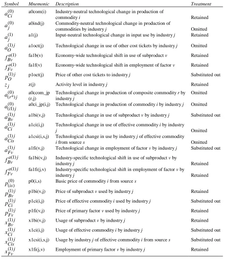
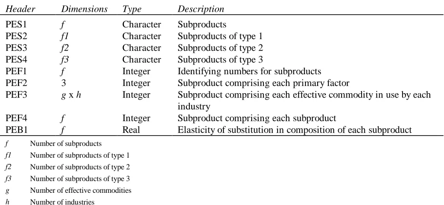
Table 1 shows the mnemonics used in the TABLO source code in the initial implementation for the variables in the production structure. It also shows the treatment of these variables in the condensation phase of TABLO. The ordering of variables in the table is first into vector variables (variables with just one index) and matrix variables (variables with two or more indices), and then alphabetically. Table 2 lists the arrays added to the invariant parameters file in the database.

Table 1: Production-related variables with flexible nesting: mnemonics and

treatment in condensation

Symbol Mnemonic Description Treatment

a_Ci( )0 a0com(i) Industry-neutral technological change in production of

commodity i Retained

a( )_j0 a0ind(j) Commodity-neutral technological change in production of

commodities by industry j Omitted

a( )_j1 a1(j) Input-neutral technological change in input use by industry j Retained

a_O( )1j a1oct(j) Technological change in use of other cost tickets by industry j Omitted

f_Bva( )1 fa1b(v) Economy-wide technological shift in use of subproduct v Retained

f_Fva( )1 fa1f(v) Economy-wide technological shift in employment of factor v Retained

p_O( )1 j p1oct(j) Price of other cost tickets to industry j Substituted out

z_j z(j) Activity level in industry j Retained

a_{( *)}( )_r0 _j a0ccom_jp

(r,j)

Technological change in production of composite commodity r by industry j

Omitted

a_{( )}( )_{i j}0₁ a0ci_jp(i,j) Technological change in production of commodity i by industry j Omitted

a_Bv( )1j a1bi(v,j) Technological change in use of subproduct v by industry j Substituted out

a_Ci( )1j a1ci(i,j) Technological change in use of effective commodity i by industry

j Omitted

a_Cis( )1j a1csi(i,s,j) Technological change in use by industry j of effective commodity

i from source s Omitted

a_Fv( )1j a1fi(v,j) Technological change in employment of factor v by industry j Substituted out

f_Bva( )1 j fa1bi(v,j) Industry-specific technological shift in use of subproduct v by

industry j Retained

f_Fva( )1 j fa1fi(j,v) Industry-specific technological shift in employment of factor v by

industry j Retained

p_{( )}( )_is0 p0(i,s) Basic price of commodity i from source s

p_Bv( )1 j p1bi(v,j) Price of subproduct v used by industry j Retained

p_Ci( )1 j p1ci(i,j) Price of effective commodity i used by industry j Substituted out

p_Fv( )1 j p1fi(v,j) Price of primary factor v used by industry j Retained

x_Bv( )1 j x1bi(v,j) Usage of subproduct v by industry j Retained

x_Ci( )1 j x1ci(i,j) Usage of effective commodity i by industry j Substituted out

x_Cis( )1 j x1csi(i,s,j) Usage by industry j of effective commodity i from source s Substituted out

Table 2: Arrays added to the invariant parameters file for the flexible nesting treatment

Header Dimensions Type Description

PES1 f Character Subproducts

PES2 f1 Character Subproducts of type 1 PES3 f2 Character Subproducts of type 2 PES4 f3 Character Subproducts of type 3

PEF1 f Integer Identifying numbers for subproducts PEF2 3 Integer Subproduct comprising each primary factor

PEF3 g x h Integer Subproduct comprising each effective commodity in use by each industry

PEF4 f Integer Subproduct comprising each subproduct

PEB1 f Real Elasticity of substitution in composition of each subproduct

f Number of subproducts

f1 Number of subproducts of type 1

f2 Number of subproducts of type 2

f3 Number of subproducts of type 3

g Number of effective commodities

h Number of industries

Note: In arrays PEF2-PEF4, elements corresponding to direct inputs into the top level of the production structure are set at zer o.

This problem can be avoided by specifying the option ‘IZ1’, ‘Ignore zero coefficients in step 1’, in running the TABLO-generated program. With this option selected, coefficients to which zero values are assigned by formulae are omitted from the equations file. This has the disadvantage in multi-step simulations of increasing the risk of failure in reusing pivots, with consequent time penalties (Harrison and Pearson 1993b p. 5-9 f.). On the other hand it greatly reduces the disk requirement for simulations with the flexible substitution treatment, and greatly accelerates the first step of the simulation.

Activity level

Leontief 0

Factor-energy bundle

N on-energy commodity 1

N on-energy

commodity g - c O ther costs

La bour

Capital-energy bundle

D omestic

product Imports CES

4 _CES

CES _CES

3

La bour type 1 La bour type M Energy

CES 1

CES 2 Capital-land

bundle

Capital La nd Energy carrier 1 Energy carrier c Figure 2: Pro duction structure in a version of O RANI-E

g Number of commodities

c Number of energy carriers

M Number of occupations

4.

Illustrative application

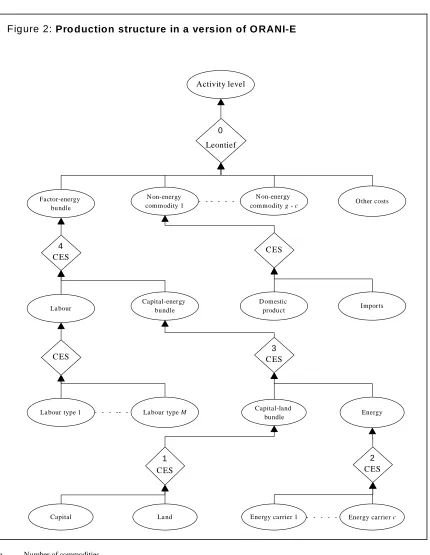
The initial application of the flexible nesting treatment was to a version of ORANI-E incorporating a disaggregated treatment of fossil fuels (Adams and Dixon 1992). We used the flexible nesting treatment to incorporate inter-fuel and energy-capital substitution.

The enhanced production structure is shown in figure 2. It involves four subproducts:

(1) a capital-land bundle composed of two primary factors, capital and agricultural land;

(2) an energy bundle composed of several effective commodities (for most industries these are

black coal, liquefied petroleum gas, natural gas, brown coal (briquettes), brown coal (lignite), petroleum and coal products, electricity, and reticulated gas);

(3) a capital-land-energy bundle composed of two subproducts, the capital-land bundle and the

energy bundle, and

(4) a factor-energy bundle composed of one factor, effective labour, and one subproduct, the

capital-land-energy bundle.

Subproduct 1 is of type one since it comprises only primary factors. Subproduct 2 is also of type one since it comprises only effective commodities, namely some industry-specific selection of energy carriers (although figure 2 does not show their composition, these energy carriers like other effective commodities in the model are composed from domestic and imported varieties). These two subproducts accordingly are included in the aray PES2. Subproduct 3 is of type two since it comprises subproducts of type two but no subproducts of higher type. Subproduct 4 is of type three since it comprises a subproduct of type three but no subproduct of higher type. Subproducts 3 and 4 are included in the arrays PES3 and PES4 respectively.

In the array PEF2 the first factor, ‘effective labour’, is assigned to subproduct 4, the energy-capital bundle, and the remaining factors ‘energy-capital’ and ‘agricultural land’ are assigned to subproduct 1, the capital-land bundle.

In the array PEF4 we assign the capital-land bundle and the energy bundle to subproduct 3, the capital-land-energy bundle. We assign the capital-land-energy bundle to subproduct 4, the factor-energy bundle. We set the entry for the factor-factor-energy bundle equal to zero, indicating that it enters directly into the top level of the production system.

In the array PEB1 we set substitution elasticities for the various subproduct aggregator functions. The elasticity settings are based on those used in the Industry Commission’s ORANI-Greenhouse model (IC 1991).

References

Adams, P.D. and Dixon, P.B. 1992, Disaggregating Oil, Gas and Brown Coal, Monash University Centre of Policy Studies mimeo.

Dixon, P.B., Parmenter, B.R., Pearson, K.R., McDonald, D., Horridge, M., and Adams, P. 1992,

The MONASH Model, paper presented to the 21st Conference of Economists, University of

Melbourne, 8 July.

Dixon, P.B., Parmenter, B.R., Sutton, J., and Vincent, D.P. 1982, ORANI: A Multisectoral

Model of the Australian Economy, North-Holland, Amsterdam.

Hanoch, G. 1971, ‘CRESH Production Functions’, Econometrica vol. 39, pp. 695-712.

Hanslow, K. 1992, Substitution between Intermediate Inputs and Primary Factors in ORANI, Industry Commission Research Memorandum No. OA-587, July.

Harrison, J. and Pearson, K. 1993a, An Introduction to GEMPACK, GEMPACK Document No. 1, Monash University IMPACT Project.

Harrison, J. and Pearson, K. 1993b, User’s Guide to TABLO and TABLO-Generated Programs, GEMPACK Document No. 2, Monash University IMPACT Project.

Appendix 1: Additions to the TABLO source code for the flexible

nesting treatment

!****************************************************************************! ! SETS ! !****************************************************************************! !============================================================================! ! SETS SHARED WITH THE STANDARD MODEL ! !============================================================================! SET COM # Commodities # (C1 - C119);

SET IND # Industries # (I1 - I117);

SET FAC # Primary Factors # (labour,capital,land);

SET COMPCOM # Composite Commodities# (cc1,cc2,cc3,cc4,cc5,cc6); SET SOURCE # Domestic/Imported # ( domestic,imported );

SET IND_UP # Unique-Product Industries # (I8 - I117); SET IND_JP # Joint-Production Industries # (I1 - I7);

!============================================================================! ! SETS ADDED FOR THE FLEXIBLE NESTING TREATMENT ! !============================================================================! ! The following sets define the subproducts used to describe the nesting structure of the production functions. !

SET SPR # subproducts # MAXIMUM SIZE 4

READ ELEMENTS FROM FILE PARAMS HEADER "PES1"; SET SPRO1 # subproducts of type 1 # MAXIMUM SIZE 2 READ ELEMENTS FROM FILE PARAMS HEADER "PES2"; SUBSET SPRO1 IS SUBSET OF SPR;

! A subproduct is of type 1 if it is composed only of factors and commodities. !

SET SPRO2 # subproducts of type 2 # MAXIMUM SIZE 1 READ ELEMENTS FROM FILE PARAMS HEADER "PES3"; SUBSET SPRO2 IS SUBSET OF SPR;

! A subproduct is of type 2 if

(1) it is not of type less than 2, and

(2) it is composed only of factors, commodities, and subproducts of type

less than 2. ! SET SPRO3 # subproducts of type 3 # MAXIMUM SIZE 1

READ ELEMENTS FROM FILE PARAMS HEADER "PES4"; SUBSET SPRO3 IS SUBSET OF SPR;

! A subproduct is of type 3 if

(1) it is not of type less than 3, and

(2) it is composed only of factors, commodities, and subproducts of type

less than 3. ! ! The following set is used for convenience in demand equations having two

SET DUMMY_INDEX SIZE 1;

!****************************************************************************! ! VARIABLES ! !****************************************************************************! !============================================================================! ! VARIABLES SHARED WITH THE STANDARD MODEL ! !============================================================================! ! VECTOR VARIABLES IN ALPHABETIC ORDER !

(ALL,j,IND) a1(j) # All Input Augmenting Technical Change #; (ALL,j,IND) a1oct(j) # "Other Cost" Ticket Augmenting Techncal Change#; (ALL,j,IND) x1oct(j) # Demand for "Other Cost" Tickets #; (ALL,j,IND) z(j) # Activity Level or Value-Added #; ! MATRIX VARIABLES IN ALPHABETIC ORDER : GENERALLY SUBSTITUTED OUT !

(ALL,i,COM)(ALL,j,IND)

a1ci(i,j) # Input i technical change - prod.#; (ALL,v,FAC)(ALL,j,IND)

a1fi(v,j) # tech. change in employment of factor v by industry j #; (ALL,i,COM)(ALL,s,SOURCE)(ALL,j,IND)

a1csi(i,s,j) # Input is technical change - prod.#; (ALL,i,COM)(ALL,s,SOURCE)(ALL,j,IND) p1csi(i,s,j) # Prices for current production #;

(ALL,j,IND)(ALL,v,FAC)

p1fi(j,v) # price / price index for factor v employed by industry j #; (ALL,i,COM)(ALL,s,SOURCE)(ALL,j,IND)

x1csi(i,s,j) # Demands for inputs for current production #; (ALL,j,IND)(ALL,v,FAC)

x1fi(j,v) # employment of factor v by industry j #;

!============================================================================! ! VARIABLES ADDED FOR THE FLEXIBLE NESTING TREATMENT ! !============================================================================! VARIABLE

! VECTOR VARIABLES IN ALPHABETIC ORDER !

(ALL,u,SPR) fa1b(u) # ind.-gen. tech. shift for use of subproducts #; (ALL,v,FAC) fa1f(v) # ind.-gen. tech. shift for use of factors #; ! MATRIX VARIABLES IN ALPHABETIC ORDER : GENERALLY SUBSTITUTED OUT !

(ALL,u,SPR)(ALL,j,IND)

a1bi(u,j) # tech. change in use of subproduct u by industry j #; (ALL,i,COM)(ALL,j,IND)

a1ci(i,j) # Input i technical change - prod.#; (ALL,u,SPR)(ALL,j,IND)

fa1bi(u,j) # ind.-specific tech. shift for use of subproduct u by industry j #; (ALL,j,IND)(ALL,v,FAC)

fa1fi(j,v) # technical shift for employment of factor v by industry j #; (ALL,u,SPR)(ALL,j,IND)

(ALL,j,IND)(ALL,v,FAC)

p1fi(j,v) # price / price index for factor v employed by industry j #; (ALL,u,SPR)(ALL,j,IND)

x1bi(u,j) # intermediate usage of subproduct u by industry j #; (ALL,i,COM)(ALL,j,IND)

x1ci(i,j) # intermediate usage of effective commodity i by industry j #; (ALL,j,IND)(ALL,v,FAC)

x1fi(j,v) # employment of factor v by industry j #;

!*****************************************************************************! ! READS FROM PARAMS FILE IN ALPHABETICAL ORDER ! !*****************************************************************************! !============================================================================! ! COEFFICIENTS SHARED WITH THE STANDARD MODEL ! !============================================================================! COEFFICIENT (ALL,i,COM) SIGMA1(i)

# Source substitution elasticity in intermediate usage of commodity i #; !============================================================================! ! COEFFICIENTS ADDED FOR THE FLEXIBLE NESTING TREATMENT ! !============================================================================! COEFFICIENT (INTEGER) (ALL,u,SPR) IDSPR(u)

# identifying number for subproduct u #; READ IDSPR FROM FILE PARAMS HEADER "PEF1"; COEFFICIENT (INTEGER) (ALL,v,FAC) NESTFAC(v) # nest containing factor v #;

READ NESTFAC FROM FILE PARAMS HEADER "PEF2";

COEFFICIENT (INTEGER) (ALL,i,COM)(ALL,j,IND) NESTCOM(i,j) # nest containing commodity i in use by industry j #; READ NESTCOM FROM FILE PARAMS HEADER "PEF3";

COEFFICIENT (INTEGER) (ALL,u,SPR) NESTSPR(u) # nest containing subproduct u #;

READ NESTSPR FROM FILE PARAMS HEADER "PEF4"; COEFFICIENT (ALL,u,SPR) SIGMA1B(u)

# elasticity of substitution in composition of subproduct u #; READ SIGMA1B FROM FILE PARAMS HEADER "PEB1";

!*****************************************************************************! ! COEFFICIENTS USED IN FLEXIBLY NESTED PRODUCTION ! !*****************************************************************************! !============================================================================! ! COEFFICIENTS SHARED WITH THE STANDARD MODEL ! !============================================================================! COEFFICIENT (ALL,v,FAC)(ALL,j,IND) TPURCHVAL1FI(v,j)

# expenditure on factor v by industry j #;

COEFFICIENT (ALL,i,COM)(ALL,j,IND) TPURCHVAL1CI(i,j) # expenditure on effective commodity i by industry j #;

COEFFICIENT (ALL,i,COM)(ALL,s,SOURCE)(ALL,j,ind) SOURCE_SHR1(i,s,j)

COEFFICIENT (ALL,i,COM)(ALL,j,IND) H0CI(i,j)

#Share of commodity i in total revenue of industry j#; COEFFICIENT (ALL,cc,COMPCOM) (ALL,j,IND_JP) H0CC(cc,j)

# Share of composite commodity cc in revenue of industry j #; COEFFICIENT TINY # Arbitrary small number #;

COEFFICIENT (ALL,j,IND) COSTS(j) # Total costs in industry j #;

COEFFICIENT (ALL,j,IND) OTHCOST(j) # "Other cost tickets" paid by industry j #; !============================================================================! ! COEFFICIENTS ADDED FOR THE FLEXIBLE NESTING TREATMENT ! !============================================================================! COEFFICIENT (ALL,u,SPR)(ALL,j,IND) TPURCHVAL1BI(u,j)

# value at purchasers' prices of usage of subproduct u by industry j #; FORMULA (ALL,u,SPR)(ALL,j,IND)

TPURCHVAL1BI(u,j) = 0.0;

COEFFICIENT (ALL,u,SPRO1)(ALL,j,IND) TPVAL1O1BI(u,j)

# value at purchasers' prices of usage of subproduct u by industry j #; ! for subproducts of type 1 !

FORMULA (ALL,u,SPRO1)(ALL,j,IND) TPVAL1O1BI(u,j)

= SUM(v,FAC: NESTFAC(v) = IDSPR(u), TPURCHVAL1FI(v,j)) + SUM(i,COM: NESTCOM(i,j) = IDSPR(u), TPURCHVAL1CI(i,j)); FORMULA (ALL,u,SPRO1)(ALL,j,IND)

TPURCHVAL1BI(u,j) = TPVAL1O1BI(u,j);

COEFFICIENT (ALL,u,SPRO2)(ALL,j,IND) TPVAL1O2BI(u,j)

# value at purchasers' prices of usage of subproduct u by industry j #; ! for subproducts of type 2 !

FORMULA (ALL,u,SPRO2)(ALL,j,IND) TPVAL1O2BI(u,j)

= SUM(v,FAC: NESTFAC(v) = IDSPR(u), TPURCHVAL1FI(v,j)) + SUM(i,COM: NESTCOM(i,j) = IDSPR(u), TPURCHVAL1CI(i,j)) + SUM(v,SPR: NESTSPR(v) = IDSPR(u), TPURCHVAL1BI(v,j)); FORMULA (ALL,u,SPRO2)(ALL,j,IND)

TPURCHVAL1BI(u,j) = TPVAL1O2BI(u,j);

COEFFICIENT (ALL,u,SPRO3)(ALL,j,IND) TPVAL1O3BI(u,j)

# value at purchasers' prices of usage of subproduct u by industry j #; ! for subproducts of type 3 !

FORMULA (ALL,u,SPRO3)(ALL,j,IND) TPVAL1O3BI(u,j)

= SUM(v,FAC: NESTFAC(v) = IDSPR(u), TPURCHVAL1FI(v,j)) + SUM(i,COM: NESTCOM(i,j) = IDSPR(u), TPURCHVAL1CI(i,j)) + SUM(v,SPR: NESTSPR(v) = IDSPR(u), TPURCHVAL1BI(v,j)); FORMULA (ALL,u,SPRO3)(ALL,j,IND)

TPURCHVAL1BI(u,j) = TPVAL1O3BI(u,j);

COEFFICIENT (ALL,v,FAC)(ALL,j,IND) VALNEST1FI(v,j)

# expenditure by industry j on nest containing factor v #; FORMULA (ALL,v,FAC)(ALL,j,IND)

VALNEST1FI(v,j)

COEFFICIENT (ALL,i,COM)(ALL,j,IND) VALNEST1CI(i,j)

# expenditure by industry j on nest containing commodity v #; FORMULA (ALL,i,COM)(ALL,j,IND)

VALNEST1CI(i,j)

= SUM(u,SPR: NESTCOM(i,j) = IDSPR(u), TPURCHVAL1BI(u,j)); COEFFICIENT (ALL,v,SPR)(ALL,j,IND) VALNEST1BI(v,j)

# expenditure by industry j on nest containing subproduct v #; FORMULA (ALL,v,SPR)(ALL,j,IND)

VALNEST1BI(v,j)

= SUM(u,SPR: NESTSPR(v) = IDSPR(u), TPURCHVAL1BI(u,j)); COEFFICIENT (ALL,u,SPR)(ALL,j,IND) NUMELTSPR(u,j) # number of inputs into subproduct u in industry j #; FORMULA (ALL,u,SPR) (ALL,j,IND)

NUMELTSPR(u,j)

= SUM(v,FAC: NESTFAC(v) = IDSPR(u), 1.0) + SUM(i,COM: NESTCOM(i,j) = IDSPR(u), 1.0) + SUM(v,SPR: NESTSPR(v) = IDSPR(u), 1.0); ZERODIVIDE (ZERO_BY_ZERO) DEFAULT 1.0; ZERODIVIDE (NONZERO_BY_ZERO) DEFAULT 1.0;

COEFFICIENT (ALL,v,FAC)(ALL,j,IND) RNONEST1FI(v,j)

# reciprocal of number of elements in nest containing factor v in ind. j #; FORMULA (ALL,v,FAC)(ALL,j,IND)

RNONEST1FI(v,j) = 1.0/SUM(u,SPR: IDSPR(u) = NESTFAC(v), NUMELTSPR(u,j)); COEFFICIENT (ALL,i,COM)(ALL,j,IND) RNONEST1CI(i,j)

# number of elements in nest containing commodity i in ind. j #; FORMULA (ALL,i,COM)(ALL,j,IND)

RNONEST1CI(i,j) = 1.0/SUM(u,SPR: IDSPR(u) = NESTCOM(i,j), NUMELTSPR(u,j)); COEFFICIENT (ALL,v,SPR)(ALL,j,IND) RNONEST1BI(v,j)

# number of elements in nest containing subproduct v in ind. j #; FORMULA (ALL,v,SPR)(ALL,j,IND)

RNONEST1BI(v,j) = 1.0/SUM(u,SPR: IDSPR(u) = NESTSPR(v), NUMELTSPR(u,j)); ZERODIVIDE OFF;

COEFFICIENT (ALL,v,FAC)(ALL,j,IND) SHSPRFAC(v,j)

# share of factor v in expenditure on corrg nest by industry j #; FORMULA (ALL,v,FAC)(ALL,j,IND)

SHSPRFAC(v,j) = RNONEST1FI(v,j);

FORMULA (ALL,v,FAC)(ALL,j,IND: VALNEST1FI(v,j) GT 0.0) SHSPRFAC(v,j) = TPURCHVAL1FI(v,j)/VALNEST1FI(v,j); COEFFICIENT (ALL,i,COM)(ALL,j,IND) SHSPRCOM(i,j)

# share of commodity i in expenditure on corrg nest by industry j #; FORMULA (ALL,i,COM)(ALL,j,IND)

SHSPRCOM(i,j) = RNONEST1CI(i,j);

FORMULA (ALL,i,COM)(ALL,j,IND: VALNEST1CI(i,j) GT 0.0) SHSPRCOM(i,j) = TPURCHVAL1CI(i,j)/VALNEST1CI(i,j); COEFFICIENT (ALL,v,SPR)(ALL,j,IND) SHSPRSPR(v,j)

# share of subproduct v in expenditure on corrg nest by industry j #; FORMULA (ALL,v,SPR)(ALL,j,IND)

SHSPRSPR(v,j) = RNONEST1BI(v,j);

! This treatment ensures that the demand equations for inputs into current production remain homogeneous even when VALNEST1?I(?,j) = 0.0. !

!*****************************************************************************! ! DEMANDS BY FIRMS FOR INPUTS INTO PRODUCTION ! !*****************************************************************************! EQUATION XI_EFFCOM

# E.F.4: price of effective commodity i used by industry j # (ALL,i,COM)(ALL,j,IND)

p1ci(i,j)

= SUM(s,SOURCE, SOURCE_SHR1(i,s,j)*(p1csi(i,s,j) + a1csi(i,s,j))); EQUATION INT_INP_DEM

# E.F.5: use of commodity i from source s by industry j # (ALL,i,COM)(ALL,s,SOURCE)(ALL,j,ind)

x1csi(i,s,j)

= x1ci(i,j) + a1csi(i,s,j)

- SIGMA1(i)*(p1csi(i,s,j) + a1csi(i,s,j) - p1ci(i,j)); EQUATION XI_SUBPRODUCT

# E.F.6: price of sub-product u used by industry j # (ALL,u,SPR)(ALL,j,IND)

p1bi(u,j)

= SUM(v,FAC: NESTFAC(v) = IDSPR(u), SHSPRFAC(v,j)*(p1fi(j,v) + a1fi(v,j))) + SUM(i,COM: NESTCOM(i,j) = IDSPR(u), SHSPRCOM(i,j)*(p1ci(i,j) + a1ci(i,j))) + SUM(v,SPR: NESTSPR(v) = IDSPR(u), SHSPRSPR(v,j)*(p1bi(v,j) + a1bi(v,j))); EQUATION EMPL_FACT

# E.F.7: employment of factor u by industry j # (ALL,u,FAC)(ALL,j,IND)

x1fi(j,u)

= SUM(v, SPR: IDSPR(v) = NESTFAC(u),

x1bi(v,j) + a1fi(u,j) - SIGMA1B(v)*(p1fi(j,u) + a1fi(u,j) - p1bi(v,j))); EQUATION INT_USE_EFF_COM

# E.F.8: Use of effective commodity i by industry j # (ALL,i,COM)(ALL,j,IND)

x1ci(i,j)

= SUM(d,DUMMY_INDEX: NESTCOM(i,j) = 0, z(j) + a1(j) + a1ci(i,j)) + SUM(u, SPR: IDSPR(u) = NESTCOM(i,j),

x1bi(u,j) + a1ci(i,j) - SIGMA1B(u)*(p1ci(i,j) + a1ci(i,j) - p1bi(u,j))); EQUATION INT_USE_SPR

# E.F.9: Use of subproduct u by industry j # (ALL,u,SPR)(ALL,j,IND)

x1bi(u,j)

= SUM(d,DUMMY_INDEX: NESTSPR(u) = 0, z(j) + a1(j) + a1bi(u,j)) + SUM(v, SPR: IDSPR(v) = NESTSPR(u),

!*****************************************************************************! ! PRICE SYSTEM ! !*****************************************************************************! EQUATION ZPP_INT_JP

# E.P.1A: Zero pure profits in production, joint production industries # (ALL,j,IND_JP)

SUM(i,COM,H0CI(i,j)*(p0dom(i) - a0ci_jp(i,j) - a0com(i))) - SUM(cc,COMPCOM,H0CC(cc,j)*a0ccom_jp(cc,j)) - a0ind(j) = a1(j)

+ (1.0/(TINY+COSTS(j)))

*( SUM(i,COM: NESTCOM(i,j) = 0, TPURCHVAL1CI(i,j)*(p1ci(i,j) + a1ci(i,j))) + SUM(u,SPR: NESTSPR(u) = 0, TPURCHVAL1BI(u,j)*(p1bi(u,j) + a1bi(u,j))) + OTHCOST(j)*(p1oct(j) + a1oct(j)));

EQUATION ZPP_INT_UP

# E.P.1B: Zero pure profits in production, unique production industries # (ALL,j,IND_UP)

SUM(i,COM,H0CI(i,j)*(p0dom(i) - a0com(i))) - a0ind(j) = a1(j)

+ (1.0/(TINY+COSTS(j)))

*( SUM(i,COM: NESTCOM(i,j) = 0, TPURCHVAL1CI(i,j)*(p1ci(i,j) + a1ci(i,j))) + SUM(u,SPR: NESTSPR(u) = 0, TPURCHVAL1BI(u,j)*(p1bi(u,j) + a1bi(u,j))) + OTHCOST(j)*(p1oct(j) + a1oct(j)));

!*****************************************************************************! ! TECHNOLOGICAL CHANGE ! !*****************************************************************************! EQUATION TECH_SHIFT_FAC

# E.TE.1: Technological change in employment of factor v by industry j # (ALL,v,FAC)(ALL,j,IND)

a1fi(v,j) = fa1f(v) + fa1fi(j,v); EQUATION TECH_SHIFT_SPR

# E.TE.2: Technological change in use of subproduct u by industry j # (ALL,u,SPR)(ALL,j,IND)

Appendix 2: Energy sectors in a version of ORANI-E

Sector

Commodity number

Industry number

Black coal 16 14

Natural gas 18 16

Liquefied petroleum gas, natural 19 17

Brown coal (lignite) 20 18

Brown coal (briquettes) 21 19

Petroleum and coal products 62 60

Electricity 90 88

Appendix 3: Data added to an ORANI-E database to model inter-fuel

and energy-capital substitution with the flexible nesting

treatment

2

ARRAY PES1, type 1C, long name ‘Subproducts’

ARRAY PES1 CONSISTS OF 4 CHARACTER STRINGS OF LENGTH 12

ENTRY

NO CHARACTER STRING CONTAINED IN THIS ENTRY 1 Capital-land

2 Energy 3 Cap-land-en 4 Factor-en

ARRAY PES2, type 1C, long name ‘Subproducts of type 1’

ARRAY PES2 CONSISTS OF 2 CHARACTER STRINGS OF LENGTH 12

ENTRY

NO CHARACTER STRING CONTAINED IN THIS ENTRY 1 Capital-land

2 Energy

ARRAY PES3, type 1C, long name ‘Subproducts of type 2’

ARRAY PES3 CONSISTS OF 1 CHARACTER STRING OF LENGTH 12

ENTRY

NO CHARACTER STRING CONTAINED IN THIS ENTRY

1 Cap-land-en

ARRAY PES4, type 1C, long name ‘Subproducts of type 3’

ARRAY PES4 CONSISTS OF 1 CHARACTER STRING OF LENGTH 12

ENTRY

NO CHARACTER STRING CONTAINED IN THIS ENTRY

1 Factor-en

2

ARRAY PEF1, type 2I, long name ‘Subproduct identifiers’

ARRAY PEF1 IS OF SIZE: 4 BY 1 ROW

1 1

2 2

3 3

4 4

ARRAY PEF2, type 2I, long name ‘Nest identifiers for primary factors’ ARRAY PEF2 IS OF SIZE: 3 BY 1 ROW 1 4

2 1

3 1

ARRAY PEF3, type 2I, long name ‘Nest identifiers for commodities’ ARRAY PEF3 IS OF SIZE: 119 BY 117 COLUMN ROW 60 88 89 Other 16,18-21 0 2 0 2

62 2 2 0 2

90 2 0 2 2

91 2 2 0 2

Other 0 0 0 0

ARRAY PEF4, type 2I, long name ‘Nest identifiers for subproducts’ ARRAY PEF4 IS OF SIZE: 4 BY 1 ROW 1 3

2 3

3 4

4 0

Array of size 4, header 'PEB1',

long name ‘Elasticity of substitution, by nest’

ROW