Modelling of protein solution properties

(1)

A Thesis submitted to the University of London

for the degree of Doctor of Philosophy

by

Sabine M. Agena, M.Sc., Dipl.-Ing.

Department of Chemical & Biochemical Engineering

University College London

London, UK

(2)

(3)

Abstract

The research pursued in this work concentrates on modelling two protein solution

properties: activity coefficients and solubility. While modelling protein solubility

was the prime objective activity coefficients were considered first as deviation from

ideal solution behaviour was expected to occur for protein containing systems.

Activity coefficients of protein related compounds, amino acids and peptides, were

studied first hypothesising that these compounds represent proteins and because

activity coefficient data is documented for those compounds but not for proteins. The

predictive UNIFAC model was studied but failed, which led to examination of the

related UNIQUAC model. The objective of the work was the creation of a model

base, which was achieved. This model base was then utilised for protein containing systems.

(4)

modelled using the established framework. Furthermore, the activity coefficient data

was examined over different pH and temperature ranges, salt types and

concentrations. A qualitative comparison of the data to protein solubility results of

other researchers was pursued and used to confirm the model approach.

Having demonstrated that protein solubility was qualitatively represented through

protein activity coefficients a quantitative solubility approach was addressed next.

For two protein systems the solubility behaviour was modelled successfully as a

function of salt concentration and temperature. Findings of other researchers were

integrated into the discussion of the model results while also the calculated protein

activity coefficients were examined and a qualitative confirmation of the model was achieved.

The models used in this study for the description of two protein solution properties,

when applied to six different proteins over various pH and temperature ranges, salt

types and concentrations showed qualitative and quantitative success. They should

(5)

Acknowledgements

I would like to express my sincere gratitude to all those who provided support

throughout my work at University College London, UK and at National Aeronautics

and Space Administration, USA.

Special thanks go to Dr. D. Bogle at U.C.L. and to Dr. M. Pusey at NASA for

supporting me and my work. I would like to thank Dr. D. Bogle for advising me

during my Ph.D. program and for arranging a European research project in which I

participated for two years. Furthermore, I am very grateful to Dr. M. Pusey who

invited me to join his Biophysics research team and supported the final year of this

work.

Furthermore, I would like to thank the team members of our European Union Project

in the United Kingdom, Denmark, Austria and Spain for their co-operation and

(6)

Rasmussen in Denmark for inviting me to their department and for their support.

Special thanks go also to Prof. F. Pessoa from Brazil for many interesting

discussions. Last, I like to thank Prof. D. Winzor, Prof. P. Wills, Prof. A. Lenhoff

and Prof. H. Blanch who took the time to discuss my work.

Furthermore, I am very grateful to the European Union who granted me a personal

(7)

List of Tables

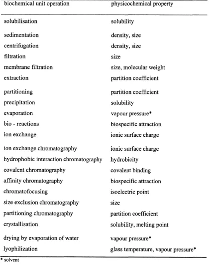
Table 1.1: Biochemical unit operations and the exploited protein properties _________ 23

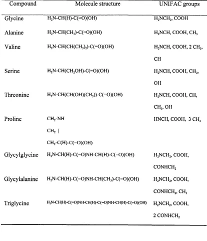
Table 2.2.1.: Molecular structure and characterisation of the twenty amino acid

residues 34

Table 2.2.2: lonised amino acid groups and their P'a and reaction_________________ 37

Table 2.4.1: The combinatorial term and residual term expressions for activity

coefficient calculations using the original UNIQUAC model _____________________ 51

Table 3.3.1.1: Molecular structures of amino acids and peptides and their UNIFAC

(12)

Table 3.3.1.2: Performance of the activity coefficient calculations for amino acids

and peptides using various IJNIFAC model versions 74

Table 3.3.2.1: Structural parameters and binary interaction parameters for glycine,

proline, glycylglycine and water 85

Table 3.3.2.2: Performance of the activity coefficient calculations for glycine, proline

and glycylglycine using the original UNIQUAC model (unsymmetric) ____________ 85

&4i&&

Table 3.3.2.3: Experirncntation error evaluation using two sets of experimentally

determined activity coefficient data for glycine, proline and glycylglycine __________ 87

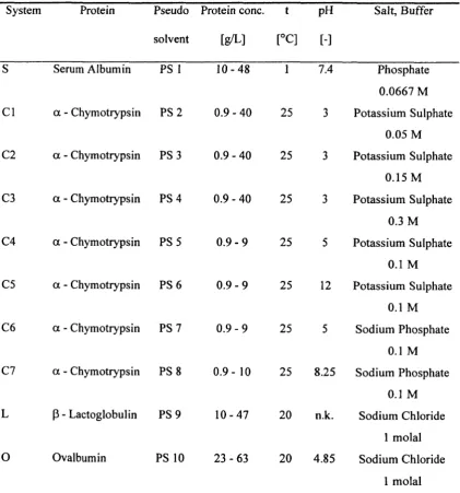
Table 4.2.1: Protein systems and system conditions investigated ____________________ 95

Table 4.2.1.1: Virial expansion data of protein systems 99

Table 4.3.1: Calculated van der Waals volumes and surface areas of proteins _______ 103

(13)

Table 4.3.3: Performance of protein activity coefficient calculations using the

original UNIQUAC model (unsymmetric) 112

Table 5.2.1: Protein systems and system conditions investigated ________________ 126

Table 5.3.1: Structural parameters of proteins, salt ions and pseudo solvents_______ 134

Table 5.4.1: Parameters of the thermodynamic solubility product for lysozyme and

concanavalin A 137

Table 5.4.2: Binary interaction parameters for the lysozyme system _____________ 139

Table 5.4.3: Binary interaction parameters for the concanavalin A system__________ 139

Table 5.4.4: Performance of solubility calculations for lysozyme and concanavalin A

using the solid - liquid equilibrium model 145

Table A. 1: Experimentally determined activity coefficients of amino acids as a

(14)

Table A.2: Experimentally determined activity coefficients of peptides as a function of

composition 182

Table C. 1: Experimentally determined activity coefficients of serum albumin, S, as a

function of composition 214

Table C.2: Experimentally determined activity coefficients of a - chymotrypsin, Cl, as

a function of composition 215

Table C.3: Experimentally determined activity coefficients of a - chymotrypsin, C2, as

afunction of composition __________________________________________________ 215

a function of composition 216

Table C.5: Experimentally determined activity coefficients of a - chymotrypsin, C4, as

Table C.6: Experimentally determined activity coefficients of a - chymotrypsin, CS, as

(15)

afunction of composition _________________________________________________ 218

Table C.9: Experimentally determined activity coefficients of J3 - lactoglobulin, L, as a

Table C.1O: Experimentally determined activity coefficients of ovalbumin, 0, as a

Table D. 1: Experimental solubility data of lysozyme, LYS, as a function of

composition and temperature 221

Table D.2: Experimental solubility data of concanavalin A, CON, as a function of

(16)

List of Figures

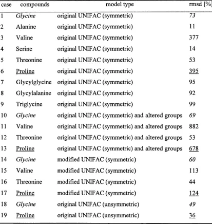
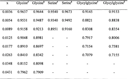
Figure 3.3.1 .1: Experimentally determined and modelled (original IINTFAC

unsymmetric) activity coefficients of glycine and proline against the amino acid and

peptide mole fraction 79

Figure 3.3.2.1: Experimentally determined and modelled (original UNIQUAC

unsymmetric) activity coefficients of glycine, proline and glycyiglycine against

theamino acid and peptide mole fraction _____________________________________ 86

Figure 4.2.1 .1: Reduced osmotic pressure of the serum albumin system against

protein concentration 98

Figure 4.3.1: The structural parameters of lysozyme, serum albumin, a

(17)

Figure 4.3.2: Programming structure used to determine interaction parameters _____ 110

Figure 4.3.3: Experimentally determined and modelled (original UNIQUAC

unsymmetric) activity coefficients of a - chymotrypsin with varying ionic strength of

potassium sulphate against protein mole fraction 114

Figure 4.3.4: Experimentally determined and modelled (original UNIQUAC

unsymmetric) activity coefficients of a - chymotrypsin with varying pH and salt

types against protein mole fraction 115

Figure 4.3.5: Experimentally determined and modelled (original UNIQUAC

imsymmetric) activity coefficients for a - chymotrypsin at different temperatures

against protein mole fraction ₁₁₆

Figure 5.2.1: Experimental solubility of lysozyme at various sodium chloride

concentrations against temperature ₁₂₈

Figure 5.2.2: Experimental solubility of concanavalin A at various ammonium

(18)

Figure 5.3.1: Structure of the solubility model 131

Figure 5.4.1: Experimental and modelled solubility of lysozyme at five different

sodium chloride concentrations against temperature 142

Figure 5.4.2: Experimental and modelled solubility of concanavalin A at different

ammonium sulphate concentrations against temperature 143

Figure 5.4.3: Modelled activity coefficients of lysozyme at different sodium chloride

(19)

Chapter 1 Modelling of Protein Solution Properties

The motivation for this work is presented and the development and pursuit of the

research project is described while the relevant publications are reviewed

1.1 Introduction

This work concentrates on the modelling of protein solution properties. Proteins were

the targeted compounds as they are a main product range in the rapidly developing

biochemical industry. From biochemical processes various proteins are produced e.g.

enzymes used in washing powders, hormones such as insulin used for medical

(20)

Two kinds of solution properties were studied for different proteins: activity

coefficients and solubility. The process of selecting these protein properties in order

to study and model them are presented in this chapter, chapter one, while also the

overall significance of this work is elaborated.

This work was pursued due to the fact that knowledge of protein solution properties,

either from experiment or from models, is of importance in a variety of areas such as

biochemical process development, protein crystal growth and medical research. The

area of optimal process development, where e.g. product quality, processing cost and

process controllability determine an optimal process, was the main focus for this

work [Bogle et al.,1996] and guided this work. In order to develop optimal biochemical processes, which is becoming increasingly important due to rising

industrial competition, the properties of the different compounds, i.e., product and

impurities, have to be evaluated. Already the first step towards the optimal process

development, which deals with the selection and arrangement of process units, i.e.,

process synthesis, requires extensive assessment of compound properties. Process

synthesis concepts have been discussed and applied with success for chemical

engineering purposes [Siirola and Rudd, 1971; Barnicki and James, 1990; Jaksland et

(21)

Wheelwright (1987) discussed applications of process synthesis concepts for

biochemical processes. He introduced heuristics based on physicochemical

compound properties. Key properties of the product, e.g. protein, and the impurities have to be screened, and those properties that demonstrate greatest difference for

product and impurities determine, which separation and purification processes are

chosen. Asenjo (1990) introduced an expert system that allows for computer aided

synthesis of biochemical processes. He also introduced a set of heuristic rules to

select process units as a function of physicochemical properties of the different

compounds or systems, e.g. bacterial cells, occurring during processing. In 1996 Wai

et al. studied a related concept using a property ratio matrix to create initial process

alternatives that are likely to lead to the optimal process.

All the mentioned synthesis methodologies require a diverse range of compound

properties as do any of the other process development stages such as process design

and process simulation. The properties needed for these methodologies are most

conveniently obtained from models and it is the aim of this research project to study

models that estimate compound properties over system conditions and predict

properties over different compound types.

(22)

process synthesis, towards the development of optimal biochemical processes, the

major process units and the relating compound properties exploited in these units

were examined. This was pursued in an attempt to screen the properties for their

importance. Protein production units used in the downstream processing from

homogenisation, solubilisation to freeze - dying were viewed with respect to the

exploited physicochemical properties and are listed in table 1 .1. Depending on the

unit operation different properties are exploited e g. an ion exchange unit is applied when differences in the ionic surface charges are found at given system conditions

for product and impurities. Likewise, e.g. sedimentation is applied as a separation

step if density and size differences are encountered for product and impurities. The

main physiochemical properties exploited in the most commonly used biochemical

unit operations are: solubility, density, size, molecular weight, partition coefficient,

biospecific attraction, ionic surface charge, hydrophopicity, covalent binding,

isoelectric point, melting point and glass temperature [Wheelwright, 1987; Burgess,

1988; Asenjo, 19901.

The decision to focus on protein solubility followed various reasons: occurrence of

solubility related unit operations in the downstream processing, the availability of

experimental data, and the non availability of an estimation or prediction method.

(23)

Table 1.1: Biochemical unit operations and the exploited protein properties

biochemical unit operation physicochemical property

solubilisation sedimentation centrifugation filtration membrane filtration extraction partitioning precipitation evaporation bio - reactions ion exchange

ion exchange chromatography

hydrophobic interaction chromatography covalent chromatography

affinity chromatography chromatofocusing

size exclusion chromatography partitioning chromatography crystallisation solubility density, size density, size size

size, molecular weight partition coefficient partition coefficient solubility

vapour pressure* biospecific attraction ionic surface charge ionic surface charge hydrobicity covalent binding biospecific attraction isoelectric point size partition coefficient solubility, melting point drying by evaporation of water vapour pressure*

(24)

[Hofmeister, 1888, and references within; Ducruix and Giege, 1992, and references

within] until today emphasises its importance. The importance to model a protein's

solubility is further demonstrated by the fact that solubility differences of compounds

are exploited in 80 % of the applied isolation procedures [Scopes, 19871 and in 57 %

of the large scale processes [Bonnerjea et al., 1986]. Furthermore, only recently

useful experimental data for protein solubility as a function of salt concentration,

temperature and p1-I [Cacioppo et al., 1991; Ewing Ct at., 1994] was made available,

which therefore allows for comprehensive modelling to be undertaken. Moreover, a

model for protein solubility, that is applicable for process development purposes, is

not yet available.

This work was motivated by the requirements for optimal biochemical process

development where e.g. a solubility model supports the design of a crystallisation

unit or can clarify if a solid and liquid phase are encountered for a certain unit

operation. However, not only engineering and production purposes link up to this

work but also studies aiming at the protein crystal growth process and at medical

research. For the protein crystal process a protein's solubility is a major property

which once it can be modelled or predicted will support the creation of crystals. To

understand a protein's crystallisation process, which is directly related to a protein's

(25)

various teams [Ducruix and Giege, 1992, and references within]. Crystals are needed

to determine a protein's three dimensional structure. Knowledge of a protein's three

dimensional structure not only enlightens our understanding of a protein's function

and biological purpose but also guides us when designing drugs.

The three dimensional description for human serum albumin [Carter et al., 1989; He

and Carter, 1992] was established as a result of such crystallisation work. Human

serum albumin carries important drugs such as aspirin in the blood and its structural

information will allow for further and enhanced drug creations and especially for

those drugs that need to be transported via the blood. Creation of the three

dimensional model of canavalin [McPherson and Rich, 1973; McPherson and

Spencer, 1975], a protein found in the jack bean and a major source of protein for

humans and domestic animals, will allow us to produce plants that are more

nutritional arid resistant to pest. Furthermore, protein crystal growth research is

applied to learn how elastase damages lung tissue while general research towards the

medical treatment for cancer, AIDS, diabetes, sickle cell anaemia and rheumatoid

arthritis is supported.

However, a precondition for this kind of work is that protein crystals are obtained but

(26)

experimental trials are encountered due to long periods of nucleation and growth

[Blundell and Johnson, 1976; McPherson, 1982], which might last over months. For

the enzyme lysozyme crystallisation periods of well above a month are encountered

when e.g. hexagonal crystals are produced [communication with Pusey, 1997]. A

method to model or even predict crystallisation conditions and therefore a model that describes protein solubility, is therefore also of great interest in this research area.

This work aims at a model for protein solubility. Models that describe protein

solubility are few. The most well known empirical description of protein solubility

with respect to salts as precipitant agents was introduced by Cohn in 1925 and has been extensively used and studied by others till today [Green, 1931; Dixon and

Webb, 1961; Foster et al., 1971; Niktari et al., 1989]. In 1977 a theoretically based

model followed. Melander and Horvath (1977) described protein solubility as a

function of salt concentration by relating the solubility behaviour to hydrophobic

effects. But Przybycien and Bailey (1989) showed that this model was not consistent

with their experimental solubility results. Further theoretical models were recently

presented by Chiew et al. (1995) and Kuehner et a!. (1996), who used molecular

thermodynamics to describe salt induced protein precipitation. The models

incorporate different interaction potentials to represent protein solubility and they

(27)

However, a solubility model is needed that computes quantitatively correctly the

protein solid - liquid equilibrium for a variety of protein systems and has a predictive

potential. Therefore, a semi - empirical model was approached, which had been used

with slight variations for the modelling of the solid - liquid equilibrium of organic

[Gmehling et al., 1978; Nass, 1988; Peres and Marcedo, 1994] and inorganic

compounds [Nicolaisen et al., 1993] but not for proteins. The theoretical framework

adapted for our systems of interest, protein - salt - water, uses the solubility product

to represent the equilibrium of liquid and crystal protein, while a protein's deviation

from ideal solution behaviour is also accounted for.

Proteins have been demonstrated to show high deviations from ideal solution

behaviour [Ross and Minton, 1977], which is expected due to the size difference

encountered between e.g. the protein and solvent molecule, i.e., water. Furthermore,

various different interactions occur for protein molecules, salt ions and water

molecules and create deviation from ideal solution behaviour. Therefore, the

modelling of protein activity coefficients representing the deviation from ideal

solution behaviour due to size difference and interactions was studied here. The only

previous studies aiming at protein activity coefficients are those of Ross and Minton

(1977), who studied sickle cell anaemia by means of activity coefficient examination,

(28)

proteins by interpreting the deduced virial coefficients which also led to activity

coefficient studies. Both teams based their work on the virial expansion, which gives

protein activity coefficients as a function of system composition at constant

temperature and pH. For this work another activity coefficient model was aimed at as

not only activity coefficients over system composition but also over system

temperature had to be expressed while additionally a predictive potential of the

model was an objective.

Activity coefficient models have been derived from Wilsons concept [Wilson, 1964]

to describe solution behaviour by means of local composition, which was developed from molecular thermodynamic theories [Smith and van Ness, 1987]. For a solution,

local compositions, different from the overall mixture composition, are assumed,

accounting for the short - range order and non - random orientation that result from

differences in molecular size and intermolecular forces. Three local composition

models are notable: the Wilson equation [Wilson, 1964], the Non Random Two

Liquid equation (NRTL) [Renon and Prausnitz, 1968] and UNiversal QUAsi

-Chemical model (UNIQUAC) [Abrams and Prausnitz, 1975].

The third local composition model, UNIQUAC model, was chosen for this work as it

(29)

UNIQUAC Functional - group Activity Coefficient model (UNIFAC) [Fredenslund

et al., 1975] was developed from it. The UNIFAC model is used to calculate activity

coefficients from contributions of defined structural molecular groups, which make

up the molecules in solution. This method creates a predictive tool not only over

system conditions as given with the UNIQUAC model but also over different but

related systems, i.e., compounds. The UNIQUAC and UNIFAC methods were

additionally chosen because they describe system composition and temperature.

While proteins had never been studied with local composition models, systems,

mainly hydrocarbons, that bear similarities with the protein - salt ions - water

systems studied here, were examined and have been described with some success

using these approaches.

Various small organic compounds, which share some of the polar properties with

proteins, were described via local composition models including compounds such as

amino acids and peptides [Nass, 1988; Gupta and Heidemann, 1990; Phino et al.,

1994; Peres and Marcedo, 1994], which are the structural building blocks of proteins.

Furthermore, polymers which share size and hydrophobic features with proteins have

been examined with UNIQUAC and UNIFAC related models [Kontogeorgis et al.,

1997, and references within], where the description of the solution behaviour focused

(30)

with proteins, were modelled describing activity coefficients and solubility

[Nicolaisen et al., 1993] using additionally the Debye Htickel law [Debye and

Hückel, 1923; HUckel, 1925, Debye, 19271 to describe the long range interactions of

ions at low salt concentrations. This modelling approach for simple electrolytes is

also of interest as salt ions are compounds occurring in the systems studied here.

Following these facts the IINIQUAC and UNIFAC models and their different

versions were studied here for protein containing systems.

In this work first of all amino acid and peptide systems, which are the building

blocks of proteins, were studied. In a systematic manner different UNIFAC and

UNIQUAC models were applied to model activity coefficients for amino acids and

peptides. This part of the work was used, to clarify if the predictive UNIFAC model

is applicable for protein related compounds and to establish which model version

would be appropriate if at all for proteins. This first part of this work is presented in

chapter three.

In the second part of this work protein activity coefficients were addressed. A

method to obtain protein activity coefficients from osmotic pressure measurements

was studied and the determined activity coefficient data was modelled using a local

(31)

examined. The model performance for protein activity coefficients over salt

concentration, pH and temperature was studied, while also a qualitative examination

of protein solubility was pursued. This second part of the work is documented in

chapter four.

In the third and final part of this work the directly measurable solution property,

solubility, was investigated. Protein solubility over salt concentration and

temperature was approached and described via the modelling of protein activity

coefficients. This part of the research is presented in chapter five.

Results and discussions are presented and summarised for these three parts. The

relevant theoretical background for this work is presented in the next chapter, chapter

two. Final chapters discuss the overall conclusions and future research projects,

(32)

Chapter 2 Theoretical Background

This chapter discusses proteins and their characteristics. Furthermore, it introduces

the major definitions and models that were studied in this work

The modelling of a protein solution property, protein solubility, was aimed at in this

work using activity coefficients. Consequently first of all proteins and their

characteristics are discussed. This is followed by the definitions for activity

coefficients and their two different standard states, the symmetric and unsynimetric

(33)

Gibbs energy is introduced leading to the UNIQUAC [Abrams and Prausnitz, 1975]

and UNIFAC [Fredenslund et al., 1975] expressions, which are models used to

describe activity coefficients and solution behaviour as a function of system

composition and temperature. The UNIQUAC and UNIFAC models are introduced

in detail, including the different UNIQUAC and UNIFAC versions examined in this

work. The presented theories are found to some extent in various references

[Prausnitz et a!., 1986; Smith and van Ness, 1987; Nicolaisen, 1994]. The discussion

relating to proteins is found in references such as Creighton (1984) and Lehninger

(1982).

2.2 Characterisation of Proteins

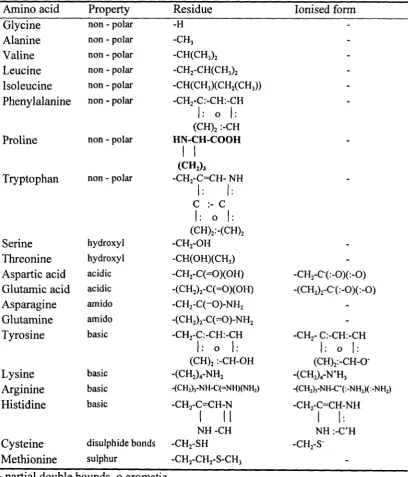
Proteins are macromolecules built from twenty natural occurring amino acids. Table

2.2.1 shows the structures of the different amino acid residues that build a particular

amino acid and are also found in proteins as amino acids are the building blocks of

proteins. These amino acid residues, R, are situated on the following structure to

configure an amino acid:

(34)

Table 2.2.1: Molecular structure and characterisation of the twenty amino acid residues

Amino acid Property Residue lonised form

Glycine non - polar -H

-Alanine non - polar -CH3

-Valine non - polar -CH(CH3)2

-Leucine non - polar -CH2-CH(CH3)2

-Isoleucine non - polar -CH(CH3)(CH2(CH3)) -Phenylalanine non - polar -CH2-C:-CH:-C1-I

-I:

o

I:

(CH)2 :-CH

Proline non - polar HN-CH-COOH

-(CH2)3

Tryptophan non - polar -CH2-CCH- NH

-C :- -C

I:

o

I:

(CH)2:-(CH)2

Serine hydroxyl -CH2-OH

-Threonine hydroxyl -CH(OH)(CH3)

-Aspartic acid acidic -CH2-C(=O)(OH) -CH2-C(:-O)(:-O) Glutamic acid acidic -(CH2)2-C(=O)(OH)

Asparagine amido -CH2-C(—O)-NH2

-Glutamine amido -(CH2)2-C(0)-NH2

-Tyrosine basic -C112-C:-CH:-CH -CH2- C:-CH:-CH

I:

o

I:

o

(CH)2 :-CH-OH (CFI)2:-CH-0

Lysine basic -(CH2)4-NH2 -(CH2)4-WH3

Arginine basic -(CH2)3-NH-C(=NH)(NH2) -(CH2),-NH-C(:-NH2)(:-NH2)

Histidine basic -CH2-C=CH-N -CH2-C=CH-NH

I

II

I

I:

NH -CII NH :-CH

Cysteine disuiphide bonds -CH2-SH -CH2-S

Methionine sulphur -CH2-CH2-S-CH3

(35)

For proline the whole structure is given in table 2.2.1 because proline is an imino

acid as opposed to an amino acid.

A protein is created from a number of amino acids which bind under a condensation

reaction resulting in a sequential arrangement:

(-NH-CH(R,j-CO-) (2.2.2)

Following these reactions a peptide or protein is created, which consists of the

backbone as given above, 2.2.2. This backbone is build of units consisting of a planar

peptide bond (-CO-NH-) and a carbon, the a - carbon, from which the particular

amino acid residue sets off. Following the condensation reactions a chain molecule is

created and its left end is defined as the amino terminus:

H2N-CH(R)-CO-... (2.2.3)

while on the other end the carboxyl terminus is found:

-NH-CH(RJ-COOH (2.2.4)

The twenty amino acids that build proteins contribute to the characteristics of

proteins. Therefore the twenty amino acids and their characteristics are discussed

next. However, amino acids do not describe matters of molecule size which have to

be additionally considered for proteins. The amino acids or amino acid residues are

(36)

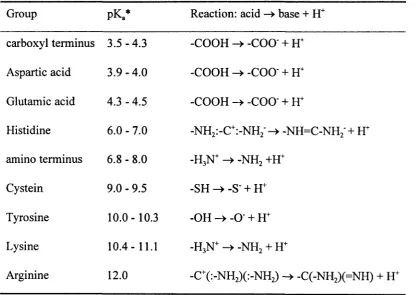
Some amino acids residues have been demonstrated to accept and release protons and

the ionised forms of these residues are given in table 2.2.1 while the acid base

reaction is documented in table 2.2.2. For six residues ionisation occurs depending

on the environment. Aspartic acid and glutamic acid release protons in the acidic pH

region and are referred to as acidic. Argine, lysine, tyrosine, cystein and histidine

(weaker base) are basic. Moreover, the termini are involved in acid base reactions.

The documented ranges for the pK., values for the different ionised groups indicate in

which pH region ionisation occurs e.g. at a pH of five the carboxyl terminus, aspartic

acid and glutamic acid are found predominantly in their base form while all other

residues are predominantly in their acid form. Following these ionisation reactions

proteins are found to be charged molecules, i.e., polyelectrolytes. In strongly acid

solution proteins are positively charged and in strongly alkaline solution they are

negatively charged. Due to this property proteins migrate in an electric field. At a net

charge of zero no migration occurs and the prevailing pH is defined as a protein's

characteristic p1 (isoelectric point).

Following the formation of ionised groups a strong hydrophilic character is observed

while the aliphatic residues participate in hydrophobic interactions. Residues such as

glycine, alanine, valine, leucine and isoleucine, table 2.2.1, exhibit a hydrophobic

(37)

Table 2.2.2: lonised amino acid groups and their pK. and reaction

Group pKa* Reaction: acid - base + H

carboxyl terminus 3.5 - 4.3

Aspartic acid 3.9 - 4.0

Glutamic acid 4.3 - 4.5

Histidine 6.0 - 7.0

amino terminus 6.8 - 8.0

-COOH -* -000 + H

-COOH - -000 + H

-COOH -^ -000 + W

-NH2 : -C:-NH2 - -NH=C-NH2 + H

-H3N -* -NH2 +W

Cystein 9.0-9.5

Tyrosine 10.0- 10.3 -OH—-O+H

Lysine 10.4-11.1 -H3N—-NH2+H

Arginine 12.0 -C(:-NH2)(:-NH2) -* -C(-NH2)(=NH) +W

* _{Creighton, 1984}

exhibits a non - polar and relatively non - reactive character. The amino acid residues

serine, threonine and tyrosine have hydroxyl groups and support hydrogen bonds.

Asparagine and glutamine, build hydrogen bonds due to their amido groups.

(38)

flexible and is often found in the bends of proteins while the steric hindered proline

limits protein flexibility. Aromatic groups found in phenylalanine, tyrosine and

tryptophan contribute to hydrophobic behaviour and steric hindrance. For cystein a very typical characteristic is the creation of disuiphide bonds, which are responsible

for strong intra- and interstrand interactions.

The interactions, which contribute mainly to the specific characteristics and structure

of a protein are the covalent bindings. Covalent linkage of atoms is established by

sharing of electrons. With covalent bonds such as the peptide bonds and the

disuiphide bonds the major characteristics of a protein's structure and therefore

characteristics are settled. An example are disuiphide bindings, which lead with increasing number to a decrease of a protein's solubility.

London dispersion forces describe short range non - covalent interactions, which also

contribute to a protein's properties. Between all atoms weak interactions occur due to

the distribution of electronic charges and their location. Their movements create

fluctuating dipoles which result in attractive forces between atoms. Repulsion occurs

when the electron orbitals are forced to overlap.

(39)

dipoles. These can lead to hydrogen bonding. Hydrogen bonding occurs for proteins

between hydrogen atoms and nitrogen atoms or hydrogen atoms and oxygen atoms.

These atoms are involved in dipole moments due to great differences in the electron density of covalent bonds. Where opposite dipole charges are found attraction occurs,

otherwise repulsion is found.

The ionic bonds, which are established between differently charged groups tend to

bring together parts over large distances while repulsion occurs between ionic groups

of same charge. Ionic bonds are the strongest non - covalent forces but do depend on

the dielectric constant of the solvent as electrostatic interactions are reduced in

solvents with high dielectric constants such as water.

When dealing with proteins another form of interaction has to be considered.

Hydrophobic interactions describe the behaviour of groups not being attracted by

water or polar substances. While polar molecule groups form hydrogen bonds with

water, non - polar groups are not soluble and tend to form hydrophobic clusters

minimising the contact area with polar solvents e.g. water, which is the solvent

proteins are most commonly exposed to. The hydrophobic parts of a protein are

accumulated in the centre while the hydrophilic parts are exposed at the surface to

(40)

for some proteins and those are referred to as globular proteins. In this work globular

proteins were studied.

Furthermore, aggregation of protein monomers occurs. Dimers or higher order

aggregates are held together by non - covalent forces as described above. During the

course of this work two proteins that occur as dimers were examined for the protein

activity coefficient and solubility modelling work, - lactoglobulin and concanavalin

A.

The described properties and interactions, which result from the molecular structure,

imply the solution behaviour that might occur between proteins and other system

compounds such as water or salt ions. Moreover, the interactions within a protein are

pictured which lead to a protein's very specific three dimensional structure unlike the

random coiling observed for aliphatic polymers.

The described structures, interactions and properties of proteins lead to certain

classifications. The most common classification is achieved by means of molecular

weights which divides the group of proteins into two groups. The low molecular

weight proteins, which are built from only a few amino acids, are referred to as

(41)

classes are defined differently with respect to the reference. One definition uses the

number of peptide bonds where a polypeptide with more than fifteen peptide bonds is

considered a protein [Freifelder, 1986]. Other references are found, which give a

definition according to the number of amino acids incorporated or the molecular

weight. Typically proteins have molecular weights of 5000 Da to 200000 Da

[Lehninger, 1982] and the average molecular weight of the amino acid, which is

incorporated into a protein and constitutes the building block of a protein, is about

120 Da [Creighton, 1984].

Furthermore, proteins are classified according to their composition [Elmore, 1986].

Unconjugated and conjugated proteins are referred to. The first class is composed of only amino acids as discussed here, while the second one has additional molecular

structures which are not amino acids. The group of conjugate proteins is divided into

nucleoproteins, lipoproteins, glycoproteins, chromoproteins in accordance to their prosthetic groups.

Moreover, certain properties are used to define proteins. A protein's solubility

behaviour allows for yet another categorisation. Albumins (soluble in water and

dilute solutions of salt), globulins (few soluble in water but soluble in dilute salt

(42)

glutelins (insoluble in the mentioned solvents but soluble in dilute solutions of acids

or bases) and scleroproteins (insoluble in most solvents) were defined over the years.

Another widely applied method of classification was established using a protein's

biological function. Such categories are hormones, enzymes, antibodies, structural

proteins etc. Since the first creation of recombinant proteins at around 1972 another

classification evolved differentiating between recombinant and non - recombinant

proteins. Furthermore, classification due to molecular size, amino acid composition,

conformation (helix content), origin and many other factors are known.

In this work six different proteins, serum albumin (horse blood), a - chymotrypsin

(bovine pancreas), - lactoglobulin (bovine milk), ovalbumin (chicken egg),

lysozyme (chicken egg) and concanavalin A (jack bean), were studied. These

proteins originate from a variety of sources as indicated above and have very

different biological functions. The protein a - chymotrypsin is a protease and its

biological function is to hydrolyse peptide bonds of proteins. The protein lysozyme,

which is the smallest protein (14600 Da) studied during the course of this work,

cleaves bacterial cell walls. Lysozyme therefore prevents infections while it is also

applied on the biochemical processing scale as a biochemical tool to disrupt bacterial

(43)

blood and regulates its osmotic pressure while it also is a transport vehicle that

delivers other compounds and drugs through the blood stream. Not only the

biological function of the studied proteins differs but also the examined system

conditions differ e.g. pH and temperature ranges. However, all these proteins have in

common that they are globular proteins, i.e., of a compact structure. Furthermore,

they all originate from natural sources that produce them at high amounts, which

makes them available at the quantities and qualities needed for biophysical studies.

Therefore, these six proteins could be studied here in the first place. The two

proteins, 3 - lactoglobulin and concanavalin A, were studied to represent proteins

that are dimers. The protein concanavalin A is the biggest protein studied here with a

molecular weight 102668 Da.

2.3 Activity Coefficients and Standard States

To model a protein's solution properties such as solubility the activity coefficients

have to be addressed. A description of a solution property has to consider the

deviation from ideal solution behaviour which is expressed through activity

(44)

is expected as demonstrated by Ross and Minton (1977) for haemoglobin.

Activity coefficients are used to describe a compound's deviation from ideal

behaviour while referring to ideal solution behaviour. Two means of referring to the

ideal solution behaviour are known and the fugacity, f, is used to define these. The

fligacity of a compound, i, in solution is represented by a product of activity, a, and

the reference fugacity:

(2.3.1)

The reference fugacity, f', is defined independently for different solution

compounds and two reference states are used: Raoult's law behaviour and Henry's

law behaviour. For Raoult's law behaviour = f (T, P, pure i) refers to the fact that

the partial pressure, p. is proportional to a compound's vapour pressure, pS:

(2.3.2)

where x is the mole fraction. The reference fugacity for Henry's law behaviour is

f ref

= H 1 and the Henry constant, H, is proportional to the partial pressure:

p1 =x1 . H1 (2.3.3)

Both laws refer to ideal solution behaviour and were found to describe the ideal

solution behaviour of different systems satisfactorily, e.g. benzene - toluene is

(45)

behaviour is only observed for mixtures of similar compounds, which are of the same

molecular size and exhibit the same interactions. Other systems exhibit deviation

from ideal solution behaviour, which has to be accounted for with reference to ideal

behaviour.

For a compound for which the standard state is the pure liquid, the activity, a, in the

standard state is equal to unity. In these cases the standard fugacity, fD, is equal to:

Jo

fref pS

(2.3.4-5)

It follows for the chemical potential, .t, that:

u,(T,P)=,u,°(T,P)+R• T . ln(a,) (2.3.6)

where a —+ 1 and .t —+ as x —+ 1 which refers to Raoult's law and introduces the

symmetric reference system. For Henry's law a hypothetical standard state is created

where the compound's activity is equal to one in pure solvent, which introduces the

unsymmetric reference state with a 1 —+ 1 as x 1 —* 0.

The activity is defined as the product of a compound's concentration and activity

coefficient, y. Different concentration scales lead to different activity and activity

(46)

a _u(x) _{=x. 'Y ()}I

a. _(rn) _{=m 7i(m)}_I (2.3.7-9) aI(C) =Cj _Yi(c)

where x is the mole fraction, m the molal and c the molar concentration scale.

Deviations from ideal solution behaviour are described by the activity coefficients,

which are a function of the specified standard state and the concentration scale. The

activity coefficients are denoted differently with respect to the standard state chosen.

For Henry's law behaviour, i.e., the unsymmetric convention, a special notation is

made: *• Otherwise Raoult's law behaviour, i.e., the symmetric convention, is

applied. The explicit activity coefficient expressions studied in this work are

introduced in the following chapters and the symmetric and unsymmetric activity coefficient equations are presented.

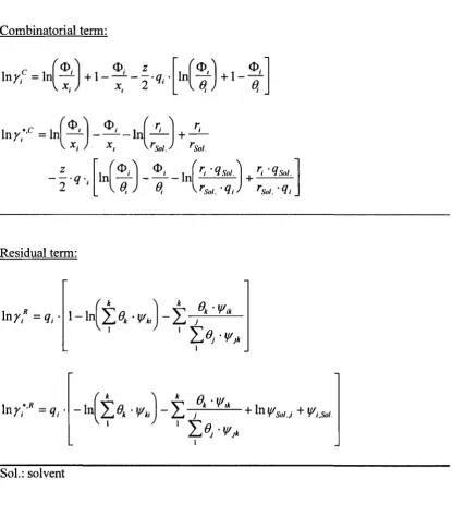
2.4. The Original UNIQUAC Model

The original UNIQUAC model [Abrams and Prausnitz, 1975] links the microscopic

and the macroscopic solution scale, creating a thermodynamic framework to describe

solution activity coefficients of pure or mixture systems over temperature. The three

dimensional arrangements and interactions of molecules as represented by lattice

(47)

means of the molar excess Gibbs energy, gE, deviation from ideal solution behaviour is described:

lny, = [(nio1 .

gE

/ R

T)1 (2.4.1)

JP,T,nj(j^i)

The activity coefficient, ', of a compound, i, is obtained by differentiating an

expression for the molar excess Gibbs energy with respect to that compound's moles,

n, while temperature, T, pressure, P. and the moles of other system compounds, j, are constant.

Exploiting the relationship given in equation 2.4.1, and aiming at the description of

phase equilibrium and furthermore equilibrium and compound properties, an excess Gibbs energy expression was introduced by Abrams and Prausnitz (1975). They

expressed the molar excess Gibbs energy as two additive terms:

gE -

g +

(2.4.2)

R•TR•T R•T

The two terms contributing to the molar excess Gibbs energy are the combinatorial

term, g, and the residual term, g.

The combinatorial term or entropy term for multi - component mixtures is given by:

E j

g c1. z

(48)

r..x q.x

and e,= 1 ' (2.4.4-5)

where

The combinatorial term accounts for deviation from ideal solution behaviour due to

differences in size and shape of the mixture compounds. The mole fraction, x, refers to

the mixture composition for all compounds, i, while the parameters (J) and 0 represent

the volume and surface fraction of the different compounds, respectively. The structural

parameters r and q refer to the volume and surface area of each compound, i.e.,

molecule, and z indicates the number of nearest neighbours, i.e., the co - ordination

number. The value, z, is generally set equal to 10 but ranges from 6 - 12 representing

the unit cell configuration of the lattice, e.g. z = 6 for the regular cubic lattice and z =

12 for the hexagonal lattice [Tanlord, 1961]. To compute the combinatorial

contribution the structural parameters, r and q, have to be determined for each system

compound. These are derived from a compound's van der Waals volume, V,, and

surface area, A, while being normalised with respect to the methylene molecular

group in polyethylene, which was an arbitrary choice by Abrams and Prausnitz

(1975):

r

= 1517 (2.4.6)

A q

(49)

To obtain a compound's van der Waals volume and surface area the group

contribution method by Bondi (1968) is generally applied. However, depending on

the compound Bondi's method might not be adequate and ways to obtain this data for

proteins were developed. These are described when relevant.

The residual term or enthalpy term is given by:

g (j

R =_q,.x,.lnIoJ .vfJI"I J (2.4.8)

( [u..—u..1

= exp— [

T (2.4.9)

With the residual term short - range interactions of a centre molecule with its ten (z)

surrounding next neighbours are introduced using binary interaction parameters, u.

Interaction parameters describe the sum of interactions between a nearest neighbour

and a centre molecule over the various binary interactions occurring per compound

pair. The interactions between identical and different molecule pairs are described by

a number of binary interaction parameters. Three interaction parameters describe for

two compounds, i and j, the binary interactions between identical, u 1 and u, and

different, u with u = ui,, compound types. The total number of binary interaction

parameters, b, needed per system is a function of the number of system compounds, i,

(50)

b = (i) + (i - l)+...+(i - i) (2.4.10)

These interaction parameters are available from previous modelling attempts for some

compounds. However, they are a function of the studied model version and might

therefore not apply. Following these facts the interaction parameters have to be

established for some compounds and this was the case for this work as proteins had not

been studied before. A programming procedure was designed and FORTRAN

programs were developed during the course of this work in order to obtain these

parameters. These procedures are explained where relevant, while the programs are

printed in the appendices.

Partial molar differentiation of the given g' expressions leads to the activity

coefficient, y, for a compound, i, over the two possible reference states, the

symmetric and unsymmetric reference states:

lny1 =lnyf+lny,' (2.4.11)

lny,* = lnr*,c + lnr* R (2.4.12)

where is the combinatorial and yR is the residual activity coefficient. In table 2.4.1

the resulting expressions are given with respect to the two terms, combinatorial and

residual term, and the two reference states, symmetric and unsymmetric conventions.

The unsymmetric activity coefficient, y, is obtained from the symmetric activity

(51)

Table 2.4.1: The combinatorial term and residual term expressions for activity

coefficient calculations using the original UNIQUAC model

Combinatorial term:

1ny14' = lnJ +1— - • q. [in-)

+1-Sc

('\ _Cj. _r _r.

in y,' = in' L _! _in ₊

x1 ) - x1 - r 01 ) rsoi

- _{q• [ln-'-J -} _-_1n"

q0j\ +

q01•

₁

r0, .q1) r 0, _•q1j

Residual term:

1ny1'=q1• 1_lfl

_f

_O

k

WkiJ -°k VIk

1

JWJk

1 [ _________

(k k

Jj

my

1

'

=q [_ifll ki - + lnsoI.,i

+i.I.1

"I

(52)

(2.4.13) V

where y defines the infinite dilution activity coefficient of a compound in pure

solvent.

2.5 The Original UNIFAC Model

Different group contribution models have been developed [Lydersen, 1955; Hoshino

et aL, 1982; Klincewicz and Reid, 1984; Mavrovouniotis et al., 1988; Mavrovouniotis,

1990; Elbro et al., 1991; Constantinou and Gani, 1994] and demonstrated that

compound properties relate not only to the molecule type but also to the molecular

groups, which build a molecule. A great variety of compounds, mainly hydrocarbons

[Lyman et aL, 1982; Reid et a!., 1987], were represented by a limited number of

molecular groups and these were successfiully correlated to a compound's molecular

structure and properties, either pure or mixture properties. These model types, group

contribution models, are able to describe properties not only of previously modelled

compounds or systems but also new and unexamined systems as the molecular

groups allow the creation of any kind of compound and therefore system. This makes

(53)

extensive and good experimental data over various conditions and systems has to be

available to develop satisfactory group contribution models, which should make the

models applicable for systems and system conditions related to the originally used

systems, i.e., systems of the database used to train the model and to obtain the needed

parameters.

Fredenslund et al. (1975) integrated such a group contribution concept into the

previously presented UNIQUAC model, chapter 2.4, and created the UNTFAC model.

The group contribution approach of the UNIFAC model uses also molecular groups, which combine to build a compound and lead to that compound's properties using the

properties of the molecular groups that build that compound. For calculations with the

UNIFAC model, as in the case of the UNIQUAC model, the structural parameters, r

and q, of a compound, i, are needed. In the case of the UNILFAC model these are

obtained from the structural parameters, R and Q, of the defmed molecular groups, p, as a function of their occurrence, v, in that same compound:

(2.5.1)

q=v . Q (2.5.2)

Two sets of structural parameters are introduced. One for the compound, r and q, and

(54)

P®.tIJ qipq)_ _/ P

I o,tIIqp

(2.5.4)

the van der Waals volume and surface area of either a compound or a molecular group

as discussed before. By means of these molecular groups and their parameters the

group contribution approach was introduced into the UNIFAC model. For the

combinatorial term of the UNIFAC model the same equations apply as for the

UNIQUAC model, equations 2.4.3 - 2.4.5, and the same theory applies as described before, chapter 2.4.

A different set of equations was derived for the residual term of the UNIFAC model.

The interaction parameters of the molecular groups, F, were integrated into the residual

term, which leads to the residual activity coefficient, y':

lny1R =v;.(lnr'-1nr';) (2.5.3)

where [ is the activity coefficient of a molecular group and F 1, is the residual activity

coefficient of group p in a reference solution containing only molecules of type i while

v refers to the number a group occurs per compound. The activity coefficient of a

molecular group is given by:

lnF

=QP{1_1n(®P

(55)

is the area fraction of a molecular group and is calculated by:

®p= qQP•XP

(2.5.5) Qq•Xq

where X is the mole fraction of a molecular group. The interaction parameter, w is

given by:

'pq

exp[

[Upq_Uqq

T j) (2.5.6)

where U is a binary interaction parameter for molecular groups and T is the system

temperature. The UNIFAC model takes the same basic approach as the UNIQUAC

model and its parameters and variables bear the same physical meaning as presented in

the previous chapter 2.4. However, for the UNIFAC model molecular groups, which

configure the different system compounds, are used as opposed to a description of the

compounds as an entity, which is done with the UNIQUAC model.

The molecular groups that are used to build a compound have been defmed and are

found in the most extensive and recent publication by Hansen et al. (1991), which also

aims at biotechnology compounds and is therefore of particular interest to this work.

Hansen et a!. (1991) defmed the molecular groups and related almost all of these

groups to the structural parameters, R and Q, and interaction parameters, U, which are a

(56)

However, reconstruction of a system's compounds using the defined molecular groups

allows for activity coefficient predictions applying the determined parameters and

introduced UNIFAC equations.

2.6 The Modified Model

In 1987 a modified model [Larsen Ct al., 19871 was developed. The combinatorial term was changed compared to the original one and was since widely used for polymers

[Kontogeorgis et a!., 1997, and references within]. Additionally, a temperature

dependence was introduced by Larsen et a!. (1987) for the residual term and its

interaction parameters. These alterations improved excess enthalpy estimations from

deviation of around 50 % to around 10 % [Fredenslund, 1989]. Consequently,

modelling of systems that span a certain temperature range can be improved using the

modified residual term. Therefore, the modified residual term was studied for this work

when temperature ranges of up to 30 K had to be described for protein solubility.

For the modified model the combinatorial activity coefficients, y, of a compound, i, is

(57)

inr,c 1J

(0.

= - +1__i (2.6.1) xi

where

2

x •r,3

= j 2 (2.6.2)

x .rJ

The modified combinatorial term is a function of the volume fraction, co, and the mole

fraction, x, and resembles closely the original combinatorial term, equation 2.4.3 and

table 2.4.1. However, the second part of the original combinatorial term is eliminated.

Due to this the entropy state of solution is described only by means of compound sizes

and reflects the originally suggested expression of Flory - Huggins [Larsen et al.,

1987].

The volume fraction of the modified model, equation 2.6.2, is determined from the

mole fractions of compounds, i and j, and relates closely to the definition given for the

original model, equation 2.4.4. However, the volume parameter, r, was assigned a

smaller contribution as examined and discussed by Kikic et a!. (1980). The introduced

exponent, which is generally and for this work set equal to 2/3, lowers the volume

contribution. The value of the exponent might vary with the type of molecule. The

structural volume parameter, r, is obtained in the manner described before, equations

(58)

The residual term of the modified model is derived in the same manner as for the

original model, chapter 2.4, but a higher order temperature dependence is added for the

binary interaction parameters, u. This results in up to three parameters per binary

interaction parameter instead of one when compared to the original model:

u = u; +u .

(T_7')+u .(T.1n-+T_7)

(2.6.3)

However, in this work the temperature, T, dependence was terminated after the second

term in order to introduce as few parameters as necessary into the solubility model. The temperature, T0, is an arbitrary reference temperature which is fixed to 300 K for this

work.

2.7 Appraisal of the Models

The basic model concepts introduced in this work are those of the UNIFAC and

UNIQUAC models. Both models refer to the same theoretical approach but vary with

the extent of their applicability. The UNIQUAC model allows for predictions over

systems conditions such as temperature and composition. The UNIFAC model

allows additionally for predictions over different but related compounds as a function

(59)

Both models have been applied to study phase equilibria and compound properties.

Pure and mixture compound properties were described for a variety of compounds by

various authors [Abrams and Prausnitz, 1975; Fredenslund et a!., 1975; Prausnitz et

at., 1986; Smith and van Ness, 1987]. The compounds investigated were mainly

hydrocarbons and small organic compounds. These relate to some degree to proteins

as discussed earlier, chapter 2.2, and therefore these models were approached.

However, some limitations are indicated for the original models as presented in 1975.

Compounds that bear an electrolyte character just like proteins, which are

polyelectrolytes, were not considered. Likewise, macromolecules such as polymers

and proteins were not included in the early examinations. However, attempts were made to overcome these limitations and since then polymers and simple electrolytes

were studied with these local composition models while this work is the first

dedicated to proteins.

For polymers it was found that a description of the entropy state of solution alone is

pursued as hardly any interactions are encountered for polymer mixtures built from

aliphatic polymers. Ways to express the entropy state of solution for polymer

mixtures were pursued using the Flory - Huggins combinatorial term as introduced

(60)

term bears also the Flory Huggins expression, it also carries a Staverman

-Guggenheim correction, which in most cases is often quite small [Larsen et al.,

1987]. For the modelling of polymer properties also variations for the definition of

the volume fraction are noted [Couthinho et al., 1994] and differences in the

definition of the volume term and the magnitude of its contribution are introduced.

These works are of relevance for protein containing systems due to the fact that they

have the macromolecular character in common with polymers. Consequently, they encouraged the study of the original models and their consecutive versions for

proteins. However, the original model and its entropy term were addressed first as

this term already introduces the size impact of the different compounds into the

model as discussed before. While for polymer solutions athermal behaviour is expected the same cannot be assumed for proteins. Having examined the

characteristics of proteins in chapter 2.2, it is for certain that interactions occur

between proteins and other system compounds. Therefore, the enthalpy state of

solution needs to be described for protein containing systems as done in this work.

Referring to the fact that proteins are polyelectrolytes, studies pursued for simple

electrolytes were of interest. Various research works have been pursued to deal with

electrolyte systems for the UNTQUAC and UNIFAC models since 1986 [Sander et

(61)

between charged groups the Debye HUckel law [Debye and I-IUckel, 1923; Huckel,

1925, Debye, 1927] was introduced. Interactions between charged groups are

observed at low ionic strength in electrolyte solutions. However, high ionic strength

solutions do not encounter charge - charge forces as these are screened off. Dealing

with protein systems that additionally constitute of buffer and salt ions, high ionic

strengths are observed and a screening of the ionic long range interactions is noted

[Kuebner et a!., 1996]. Therefore, this approach was not adapted for the studied

systems and only short - range forces such as dispersion and dipole forces were

accounted for.

Furthermore, it was of interest for this work that recently a new database of

molecular groups and their parameters [Hansen et al., 19911 was published for the

UNIFAC model, which was documented to have been extended to compounds

relevant in biotechnology applications. Success of these parameters for the prediction

of protein activity coefficients or those of related compounds is certainly of interest

for this work. The determination of parameters for the target systems would not be

required, which is a work intensive process depending on the number of parameters

that need to be determined. For the establishment of e.g. a solubility model about

twenty parameters were determined by Nicolaisen (1994) for a system of five

(62)

biotechnology compounds, was introduced for the predictive UNIFAC model

encouraged the use of the discussed modelling frameworks for biotechnology

compounds: proteins.

Consequently, first the UNIFAC model and the new database was examined. The

approaches and results of that work are discussed in the next chapter, chapter three.

This work is then followed by two further result sections which deal with additional

model approach examinations for proteins and lead to the modelling of protein

solubility.

2.8 Summary

The characteristics of proteins, major definitions and models for this work were

introduced and discussed. However, this introduction was limited to the theory

needed throughout this work and for the next chapter, chapter three. Further

(63)

a A b C Da f E g gE E gR H m n p P PT plc pS q Q R r R R

2.9 Nomenclature

activity

Van der Waals surface area

total number of binary interaction parameters molar concentration

dalton [g!molJ fugacity

combinatorial term of the molar excess Gibbs energy molar excess Gibbs energy

residual term of the molar excess Gibbs energy Henry's constant

compound

molal concentration number of moles partial pressure pressure

isoelectric point

dissociation constant on the pH scale vapour pressure

structural surface area parameter of a compound structural surface area parameter of a group gas constant

(64)

T temperature

u UNIQUAC binary interaction parameters of a compound U UNIQUAC binary interaction parameters of a group UNIFAC model UNIQUAC Functional Activity Coefficients model UNIQUAC model UNIversal QUAsi Chemical model

V Van der Waals volume

x compound mole fraction

X group mole fraction

z lattice co - ordination number

Greek letters 1' 0 '-I' 7 Il V 0 (0 '4' Subscript 0 c J

volume fraction (org.) group activity coefficient group area fraction

group interaction parameter compound activity coefficient chemical potential

molecular group occurrence per compound compound area fraction

volume fraction (mod.)

molecule interaction parameter

standard

molar concentration compound

(65)

k compound

molecular group

m molal concentration

p molecular group

q molecular group

tot total

x mole fraction

Superscript

J) infinite dilution

standard

* _{unsymmetric convention}

C combinatorial term

i compound

R residual term

ref reference

t' temperature (third term)

(66)

Chapter 3 Calculation of Amino Acid and Peptide Activity Coefficients

It was the objective of this part to evaluate which model approach describes a

solution and mixture property, activity coefficients, of amino acids and peptides.

Aiming at the description of protein solubility by means of protein activity

coefficients required first the examination of the various activity coefficient models.

The UNIFAC [Fredenslund et a!., 1975] and UNIQUAC [Abrams and Prausnitz,

1975] models and their consecutive versions were investigated for their ability to

describe activity coefficients using binary systems of amino acids arid peptides in

Modelling of protein solution properties

Abstract

Acknowledgements

Table of Contents

List of Tables

List of Figures

Chapter 1