Modeling the separation of microorganisms in
bioprocesses by flotation
Stefan Schmideder1 , Christoph Kirse1 , Julia Hofinger2, Sascha Rollié2and Heiko Briesen1,*
1
2
3
4
5
6
7
8
9
10
11
12
13
14
15
16
1 TechnicalUniversityofMunich;ChairofProcessSystemsEngineering;85354Freising,Germany 2 BASFSE;67056LudwigshafenamRhein,Germany
* Correspondence:[email protected];Tel.:+49-8161-71-3272
Abstract:Bioprocessesfortheproductionofrenewableenergiesandmaterialslackefficientseparation processesfortheutilizedmicroorganismssuchasalgaeandyeasts.Dissolvedairflotation(DAF)and microflotationarepromisingapproachestoovercomethisproblem.Theefficiencyoftheseprocesses dependsontheabilityofmicroorganismstoaggregatewithmicrobubblesintheflotationtank.In thisstudy, differentneworadapted aggregation modelsfor microbubblesand microorganisms arecomparedandinvestigatedfortheirrangeofsuitabilitytopredicttheseparationefficiencyof microorganismsfromfermentationbroths.Thecomplexityoftheheteroaggregationmodelsrange fromanalgebraicmodeltoa2Dpopulationbalancemodel(PBM)includingtheformationofclusters containingseveralbubblesandmicroorganisms.Theeffectofbubbleandcellsizedistributionsonthe flotationefficiencyisconsideredbyapplyingPBMs,aswell.Todeterminetheimpactofthemodel assumptions,themodelingapproachesarecomparedandclassifiedfortheirrangeofapplicability. Evaluatingcomputationalfluiddynamics(CFD)ofaDAFsystemshowstheheterogeneityofthe fluiddynamicsintheflotationta nk.Sinceanalysisofthestreamlinesofthetankshownegligible backmixing,theproposedaggregationmodelsarecoupledtotheCFDdatabyapplyingaLagrangian approach.
Keywords:Flotation;Separationofmicroorganisms;Bioseparation;Heteroaggregation;Population balancemodeling;CouplingofaggregationandCFD;Modelcomparison
17
1. Introduction 18
Yeast cells and algae are frequently used in bioprocesses for the production of renewable materials 19
and biofuels [1–4]. The separation of the microorganisms after fermentation is capital and energy 20
intensive. The high separation costs are caused by the small size of microalgae, their growth in very 21
dilute cultures, and their density close to that of water [5,6]. Thus, traditional separation techniques 22
such as filtration, sedimentation, and centrifugation are inefficient [7]. The development of efficient 23
separation processes is essential for the economically feasible production of renewable materials and 24
biofuels. 25
Dissolved air flotation (DAF) and microflotation are promising approaches to separate 26
microorganisms from the culture broth [6,8–10]. In both flotation principles, microbubbles (bubbles 27
with diameter ranging from 10 to 100 µm) are generated at the inlet to a flotation tank [9,11]. In the 28
flotation tank, the microbubbles and particles aggregate. The particle-bubble aggregates either float 29
into the froth of the tank or are entrained within the clear or recycle stream [12,13]. DAF is already 30
a widely used separation technique in water and wastewater treatment dealing with the removal of 31
cells, algea, and flocs of organic or inorganic materials from water [1,12,14–17]. In order to yield high 32
separation efficiencies, a pre-flocculation process with coagulants can be favorable [1,18,19]. However, 33
to avoid product damage or contamination, flocculation with coagulant should be avoided in some 34
processes [1]. 35
Applying suitable modeling approaches can significantly reduce the effort of determining efficient 36
plant configurations and process conditions for flotation. The efficiency of the separation process of 37
microorganisms with DAF or microflotation depends on the ability of microorganisms to aggregate 38
with microbubbles. To our knowledge, there exists no generic and physically correct modeling 39
approach for this heteroaggregation process. Only Zhang et al. (2014) [20] modeled the harvesting of 40
microorganisms with DAF by applying the so called “White Water Blanket Model”. They consider the 41
aggregation of several bubbles on single flocs of cells, which are polydisperse in size. However, they 42
neglected the polydispersity of bubbles and the formation of clusters consisting of several bubbles and 43
flocs. In the present study, several mechanistic approaches are taken to model the heteroaggregation 44
between microorganisms and microbubbles in flotation tanks. While still being adapted to the given 45
problem, some of the aggregation models are based on existing models for particle separation by DAF 46
[13,17,21–24]. Other modeling approaches are newly developed in this study. Each model is based 47
on different assumptions for the flotations system: averaged, i.e. homogeneous, loading of cells on 48
bubbles, distributed loading of cells on bubbles, polydispersity of cells, polydispersity of bubbles, and 49
formation of clusters with and without an averaged, i.e. homogeneous, numbers of cells and bubbles. 50
To determine the impact of the presented assumptions, the modeling approaches are compared and 51
classified for their range of applicability. Data of computational fluid dynamics (CFD) of a DAF system 52
show, that the fluid dynamics are highly heterogeneous in the flotation tank and that there is negligible 53
backmixing. Thus, the aggregation models are coupled with the CFD data of the DAF system by using 54
a Lagrangian approach. 55
2. Modeling approaches 56
In this study, six different mechanistic models for the heteroaggregation between microbubbles 57
and microorganisms dispersed in a fluid are investigated to calculate the separation efficiency of 58
microorganisms in flotation systems. The aggregation models exhibit different levels of complexity 59
and are applied for two approaches: the classical two zone model [12] with constant flow conditions 60
and the coupling to CFD data by using a Lagrangian approach. 61
2.1. Aggregation kernel 62
Each aggregation model contains the aggregation kernel β. The aggregation kernel for the
63
aggregation mechanismiis a combination of the encounter frequencyKC,iand the encounter efficiency,
64
which is the probability of an encounter leading to a successful collision [24]: 65
βi=PA,i·PC,i·KC,i, (1)
wherePA,iandPC,iare the encounter efficiencies due to physiochemical and hydrodynamic effects,
66
respectively. Commonly, the kernels for different mechanisms are superimposed [24,25]: 67
β=βL+βS+βT, (2)
whereβL,βS, andβTare the aggregation kernels due to laminar shear, sedimentation, and turbulent
68
motion. Here, aggregation due to Brownian motion can be neglected, since the cells and bubbles are 69
too large to observe Brownian motion [26]. It is well known [27,28] that an error is made with the linear 70
superimposition, but no closed form including all of the relevant mechanisms exist yet. Furthermore, 71
as the focus of this study is on comparing different models a perfect representation of the kernels is not 72
necessary. Substituting Equation (1) in Equation (2) and assuming that the physiochemical encounter 73
efficiency is independent of the aggregation mechanism, the following relation is obtained 74
Frequency of encounters 75
The frequency of encounters is calculated for each mechanism: laminar shear, sedimentation, and 76
turbulent motion. Pedocchi and Piedra-Cueva [29] have extended the frequency of encounters due to 77
laminar shear by von Smoluchowski [30] from a one dimensional formulation to a three-dimensional 78
one (Equation (4) in Table1), whereu,v, andware the fluid velocities in thex,y, andzdirections. 79
To calculate the encounter frequency due to density differences between two different aggregates, 80
Equation (5) in Table1has been used [24], wherev1andv2are the rising or settling velocities of the
81
two aggregates 1 and 2. The rising velocity of aggregates consisting of bubbles is set to the rising 82
velocity of single bubbles. For the turbulent encounter frequency, the Saffman-Turner relation is used 83
[27] (Equation (6) in Table1). 84
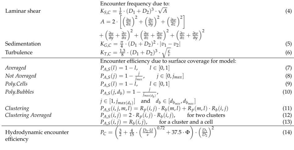
Table 1.Encounter frequencies and efficiencies used for aggregation kernels
Encounter frequency due to: Laminar shear KS,C= 16·(D1+D2)3·
√ A
A=2·
∂u ∂x
2
+∂v ∂y
2
+∂w ∂z
2
+∂u ∂y+
∂v ∂x
2
+∂u ∂z+
∂w ∂x
2
+∂v ∂z+
∂w ∂y
2
(4)
Sedimentation KG,C= π4 ·(D1+D2)2· |v1−v2| (5)
Turbulence KT,C= 1.38 ·(D1+D2)3·
q e
ν (6)
Encounter efficiency due to surface coverage for model:
Averaged PA,S(l) =1−l, l∈[0, 1] (7) Not Averaged PA,S(j) =1−jmaxj , j∈[0,jmax] (8) Poly.Cells PA,S(l) =1−l, l∈[0, 1] (9) Poly.Bubbles PA,S(j,db) =1−jmax(jdb),
j∈[1,jmax(db)] and db∈[dbmin,dbmax]
(10)
Clustering PA,S(i,j,m,l) =Rp(i,j)·Rb(m,l) +Rp(m,l)·Rb(i,j) (11) Clustering Averaged PA,S(i,j) =2·Rp(i,j)·Rb(i,j), for two clusters (12) PA,S(i,j) =Rb(i,j), for a cluster and a cell (13) Hydrodynamic encounter
efficiency
PC=
3 2+154 ·
D2·U
ν 0.72
+37.5·Φ
·D1
D2
2
(14)
Encounter efficiency 85
The hydrodynamic encounter efficiencyPCconsiders the fact that the flow field around the bubble
86
and particle hinders aggregation [31,32]. PCcan be expressed as Equation (14) in Table1, whereD1
87
andD2are the diameter of the particle and bubble,νis the kinematic viscosity of the fluid, andΦis
88
the gas volume fraction. This efficiency was derived for dirty interfaces [31,32], which is valid here, 89
because the flotation bubbles are created in a complex medium that will dirty the interface shortly after 90
bubble creation. This correlation used forPCneglects, e.g. effects of density differences [33], but again
91
the focus is not a perfect representation of the kernels but a model comparison. The characteristic 92
velocityUdepends on the aggregation mechanism. According to Kostoglou et al. [25] and Dai et al. 93
[34] the characteristic velocities for laminar shear and sedimentation are the rising velocities of the 94
bubbles. The average relative velocityUTdue to turbulent motion can be expressed as [25]
95
UT= 5
2Π·
r e
15ν ·(D1+D2), (15)
whereeis the turbulent dissipation.
96
The encounter efficiencyPA=PA,S·PA,0allows describing space limitations on the bubblePA,S
97
[13,23] or other effects such as repulsion and attractive forcesPA,0[35]. Repulsion and attractive forces
98
depend heavily on the process conditions and can be influenced by the addition of chemicals that tailor 99
by Born repulsion forces [36] or be computed using molecular dynamics simulations [37], which 101
requires knowledge of the surface of the particles, or be measured using atomic force microscopy 102
[38]. Using those methods to inferPA,0, the effect of chemical addition on separation efficiency should
103
become predictable with a suitable aggregation model. Nevertheless, most of the studies on DAF 104
estimatePA,0from empirical relations or by fitting experimental data [17,23]. Since this study describes
105
the generalized modeling of flotation processes,PA,0is set to one. Most studies on DAF processes,
106
including this one, consider that surface coverage reduces the encounter efficiency and assume that the 107
encounter efficiency is proportional to the ratio of the remaining free surface to the total surface. The 108
cells occupy their projected surface area on the bubble surface [13,17,23]. The development of layers 109
with multiple cells on the surface of bubbles is neglected in this study, since it is assumed that the cells 110
do weakly aggregate with others. If the cells would aggregate, one could easily use a coagulation unit 111
prior to flotation to increase the size of the cell-aggregates and the flotation efficiency. 112
2.2. Spatial models 113
There exist two different approaches to model the separation efficiency in DAF tanks. The 114
traditional approach divides the DAF tank into the contact zone and the separation zone [11–13,23]. 115
More advanced approaches combine CFD simulations with the aggregation process in flotation tanks 116
[24,25,39]. In this study both approaches are examined and applied to the different aggregation models. 117
Two zone model 118
It is assumed that aggregation only occurs in the contact zone, where bubbles and cells enter the 119
inlet and aggregate until the outlet of the contact zone. Since plug flow with constant flow conditions 120
is assumed, the introduced substantial derivatives for the aggregation models in Section2.3simplify 121
to time derivatives. The terms for the change of the bubble concentration over time due to velocity 122
differences between bubbles and the fluid can be neglected. Furthermore, no aggregation occurs in the 123
flotation zone and all cells, which have been attached onto bubbles in the contact zone float and are 124
thus removed. The separation efficiencyηis calculated as
125
η=1− ccoutlet
ccinlet
, (16)
whereccoutletandccinletare the concentrations of unbounded cells at the outlet and at the inlet of the
126
contact zone, respectively. 127
Lagrangian model 128
To combine CFD simulations with the aggregation process in DAF tanks, an Euler/Euler CFD 129
simulation (for the commercially available DAF system Enviplan: AQUATECTOR®Microfloat®, see 130
Figure5afor a two phase system consisting of the liquid and gaseous phase has been performed with 131
Ansys Fluent. The gaseous phase was described by bubbles with a diameter of 40 µm and a density of 132
an air bubble with a maximum loading of microorganisms (18.28 kg/m3). Those estimates were based 133
on experimental data for the flotation of yeasts (data not shown). For the liquid phase, water properties 134
were applied. The central inlet was a mass flow inlet, the free surface a degassing boundary and one 135
bottom opening (side) a pressure outlet. The mesh consisted of hexahedral cells (approximately 0,5 136
Mio. elements). Most of the tank was expected to be laminar, while the inlet region had a Reynolds 137
number in the turbulent regime. Therefore, different turbulence models (k-omega SST, k-epsilon) and 138
a model without turbulence (laminar) were evaluated but no effect on gas hold-up or flow field was 139
observed. For drag on the bubbles, the model by Tomiyama et al. [40] was used. 140
In order to combine CFD results and aggregation processes, several streamlines are tracked. While 141
unbounded cells are assumed to follow the fluid streamline until the outlet is reached, the concentration 142
of bubbles decreases on the course of a streamline due to velocity differences between bubbles and 143
derivatives and the included terms for the time dependent change of the bubble concentration. The 145
change of the bubble concentration is combined with the CFD simulations. CFD results also show that 146
unloaded bubbles and loaded bubbles behave very similar. Thus, it is assumed that free bubbles and 147
bubble-particle aggregates behave in the same way. 148
Additionally, CFD data show, that the gas volume fraction in the outlet of the flotation tank is 149
negligible (see Figure5). Assuming that bubble-cell aggregates behave like unloaded bubbles, all cells, 150
which are attached to bubbles, float. Only the unbounded cells remaining in the outlet do not float. 151
Thus, the separation efficiency for the Lagrangian model is calculated as described in Equation (16). 152
The recycling of the outlet is generally implementable in the introduced models but not included in the 153
given study. The integration of heteroaggregation processes and CFD data by the realized Lagrangian 154
approach poses a sufficient and useful method for design evaluation. Full coupling can be done in 155
a future step and might be interesting if bubble dynamics might be affected by significant change in 156
bubble density and corresponding effects on fluid dynamics. 157
2.3. Heteroaggregation modeling 158
In this section the applied models for the heteroaggregation between microbubbles and cells 159
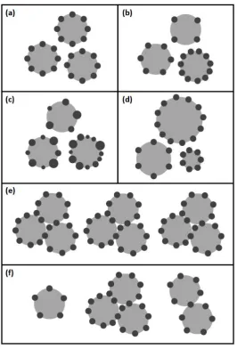
Figure 1. Illustration of the different aggregation models, where grey spheres represent bubbles and dark spheres correspond to microorganisms: (a)Averaged: several monodisperse cells aggregate on monodisperse bubbles; loading of bubbles is averaged; (b)Not Averaged: several monodisperse cells aggregate on monodisperse bubbles; loading of bubbles is distributed; (c)Poly.Cells: several polydisperse cells aggregate on monodisperse bubbles; (d)Poly.Bubbles: several monodisperse cells aggregate on polydisperse bubbles; (e)Clustering Averaged: formation of aggregates with multiple monodisperse bubbles and monodisperse cells; bubble and cell number per cluster is averaged; (f) Clustering: formation of aggregates with multiple monodisperse bubbles and monodisperse cells; bubble and cell number per cluster is distributed
Averaged 161
The modelAverageddescribes the aggregation of multiple cells on larger bubbles. Moreover, the 162
bubbles and cells are assumed to be monodisperse in their size and shape. The loading of bubbles 163
with cells is assumed to be uniform, i.e. each bubble’s surface area is occupied with cells in the same 164
manner. The general equation for aggregation between cells and bubbles is 165
Dcc
Dt =−β(dc,db,X)·cc·cb (17) whereccand cb are the number concentrations of unbounded cells, respectively bubbles, tis the
166
time, anddcanddbare the diameter of the cells and bubbles, respectively. If the conditions are not
167
X. The encounter efficiency due to surface coverage is calculated by Equation (7) in Table1, wherelis 169
the ratio of the occupied and total surface area of a bubble. Applying the Lagrangian approach, the 170
velocity difference between bubbles and the fluid causes a change of the bubble concentration on the 171
course of a streamline 172
Dcb
Dt = cb Φ ·
dΦ
dt , (18)
where the gas volume fractionΦand its time dependent change was obtained from CFD data in this 173
study. 174
Not Averaged 175
In contrast to the modelAveraged, the loading of bubbles with cells is not assumed to be uniform 176
in the modelNot Averaged, i.e. there exists a number density distribution of bubbles loaded with a 177
different amount of cells. Therefore, models where multiple bubbles can aggregate on larger particles 178
[17,21,22] have been adapted to a population balance model for the aggregation of several cells on 179
larger bubbles. Thus, a bubble withjattached cells can be formed by the aggregation between a bubble 180
withj−1 attached cells and a single cell. If a bubble withjattached cells aggregates with one more 181
cell, a bubble withj+1 cells is created. The model results in a 1D discrete population balance model, 182
in which bubbles are loaded with a discrete number of cells. 183
Dc0
Dt =−β(dc,db,j=0,X)·cc·c0+ c0
Φ·
dΦ dt Dcj
Dt =β(dc,db,j−1,X)·cc·cj−1−β(dc,db,j,X)·cc·cj (19) + cj
Φ·
dΦ
dt , j∈[1,jmax−1] Dcjmax
Dt =β(dc,db,jmax−1,X)·cc·cjmax−1+
cjmax Φ ·
dΦ dt Dcc
Dt =
jmax−1
∑
j=0
−β(dc,db,j,X)·cc·cj, (20)
whereccis the number concentration of unbounded cells andcjis the number density of monodisperse
184
bubbles loaded withjcells. The physiochemical collision efficiencyPA(j), for a bubble already having
185
jattached cells (compare with [23]) can be expressed as Equation (8) in Table1, wherejmax =
4·d2 b d2
c is 186
the maximum number of cells that can attach to a bubble. 187
Poly.Cells 188
In the modelPoly.Cells, the bubbles are still assumed to be monodisperse, whereas cells are 189
polydisperse in size. Since cells are polydisperse, the surface coverage of bubbles is continuous. Thus, 190
bubbles have the occupancy levell, which is the ratio between the occupied and total surface area of a 191
bubble. Each cell diameter is assigned a specific occupancy potentialp, which can be expressed as 192
p(dc) =
Ac,projected
Ab,sur f ace
= d
2
c
4·d2b, (21)
whereAc,projectedis the projected surface area of a cell andAb,sur f aceis the surface area of a bubble. Due
193
to a aggregation with a cell with the occupancy potentialp, the occupancy level of a bubble increases 194
froml0tol=l0+p. The set of equations for the 1D continuous population balance model is
Dcb(l)
Dt =
Z pmax
p=pmin
β(dc,db,l−p,p,X)·cb(l−p)·cc(p)dp
−cb(l)·
Z lmax−l
p=pmin
β(dc,db,l,p,X)·cc(p)dp (22)
+ cb(l)
Φ ·
dΦ
dt, l∈[0, 1]
cb(l) =0 forl<0 (23)
Dcc(p)
Dt =−cc(p)·
Z lmax−p
l=lmin
β(dc,db,l,p,X)·cb(l)dl, (24)
p∈[pmin,pmax],
wherecc(p)is the number density of polydisperse cells with the occupancy potentialpandcb(l)is
196
the number density of monodisperse bubbles with the occupancy levell. PA,Sur f aceis described in
197
Equation (9) in Table1. 198
Poly.Bubbles 199
The models by Fukushi et al. [13] and Matsui et al. [23] have been adapted to the 200
heteroaggregation between smaller monodisperse cells on larger polydisperse bubbles. That results 201
in a population balance, in which the discrete property is the loading of cells on bubbles and the 202
continuous property is the size of bubbles 203
Dc0(db)
Dt =−β(dc,db,j=0,X)·cc·c0(db) + c0(db)
Φ ·
dΦ dt Dcj(db)
Dt =β(dc,db,j−1,X)·cc·cj−1(db) −β(dc,db,j,X)·cc·cj(db) +
cj(db) Φ ·
dΦ dt Dcjmax(db)
Dt =β(dc,db,jmax−1,X)·cc·cjmax−1(db)
+cjmax(db)
Φ ·
dΦ dt
db∈[dbmin,dbmax]
j∈[1,jmax−1]
(25)
Dcc
Dt =
Z d bmax
db=dbmin jmax−1
∑
j=0
−β(dc,db,j,X)·cc·cj(db)db, (26)
wherecj(db)is the number density of bubbles with the diameterdbandjattached cells. The number
204
concentration of unbounded cells is represented ascc. The maximum number of cells that can attach
205
to a single bubblejmax(db) =
4·d2 b d2
c depends on the respective bubble diameter. The minimum and 206
maximum bubble diameter are defined asdbmin anddbmax. The encounter efficiency due to surface 207
coverage is calculated as in Equation (10) in Table1. 208
Clustering 209
The modelClusteringis based on the model by Lakghomi et al. [24], in which clusters of bubbles 210
and particles were considered. In this study clustering is the formation of aggregates with multiple 211
bubbles and cells, where both, bubbles and cells are assumed to be monodisperse. This results in a 212
DCi,j
Dt = 1 2·
i
∑
m=0
j
∑
l=0
β(dc,db,i,j,m,l,X)·Cm,l·Ci−m,j−l
−
imax−i
∑
m=0
jmax−l
∑
l=0
β(dc,db,i,j,m,l,X)·Ci,j·Cm,l
+Ci,j
Φ ·
dΦ
dt , fori>0 (27)
DC0,1
Dt =−
imax
∑
m=0
jmax−l
∑
l=0
β(dc,db,i,j,m,l,X)·C0,1·Cm,l, (28)
whereCi,j is the number density of clusters withibubbles andjcells. Contrary to Lakghomi et al.
214
[24], in this study, the reduction of the encounter efficiency due to surface coverage is included. It 215
is assumed that aggregation between two clusters can only occur, if a cell on the exposed surface 216
of a cluster collides with a bubble on the exposed surface of the other cluster or vice versa. Then 217
PA,sur f ace between a cluster withibubbles andjcells (Cluster 1) and a cluster withmbubbles and
218
lcells (Cluster 2) can be expressed as described in Equation (11) in Table1. Rp(i,j)andRb(i,j)are
219
the fractions of the exposed cluster surface area of Cluster 1 which is occupied by cells and bubbles, 220
respectively. The derivations forRpandRbare described in the AppendixB.
221
There is no suitable approach to model the hydrodynamic encounter efficiency between two 222
clusters consisting of bubbles and particles in literature. Thus, the hydrodynamic encounter efficiency 223
PCfor the case of clustering has been simplified. The expression by Kostoglou et al. [25] is used for
224
the hydrodynamic encounter efficiency of single cells and clusters consisting of one or more bubbles. 225
For two clusters, both containing one ore more bubbles, the hydrodynamic encounter efficiency is 226
predicted to be close to 1 by this model. Therefore, a value of 1 is used forPC.
227
Clustering Averaged 228
For the modelClustering Averagedit is assumed that all clusters have the same number of bubbles 229
and cells. The number concentration of free cellsccdecreases over time due to aggregation with
230
clusters, whereas the number concentration of clusterscAggdecreases due to the aggregation of two
231
clusters and due to the velocity difference between bubbles and the fluid. The average number of 232
bubbles and cells per clusteriandjcan be described as well. The product ofcAggandidoes only
233
change due to the velocity difference between bubbles and the fluid, whereas the product ofcAggandj
234
additionally increases due to the aggregation of unbounded cells. The initial number concentration of 235
clusters is equal to the initial bubble number concentration. 236
Dcc
Dt =−β(i,j,dc,db,X)·cc·cAgg (29) DcAgg
Dt =−β(i,j,dc,db,X)·c
2
Agg+
cAgg Φ ·
dΦ
dt (30)
D cAgg·i
Dt =
cAgg·i Φ ·
dΦ
dt (31)
D cAgg·j
Dt =β(i,j,dc,db,X)·cc·cAgg+ cAgg·j
Φ ·
dΦ
dt (32)
The encounter efficiency due to surface coverage between two identical cluster or between a cluster and 237
an unbounded cell can be calculated with Equation (12) and (13) in Table1. Equivalent to the model 238
Clustering, Equation (14) is used for the hydrodynamic encounter efficiency of single cells and clusters 239
consisting one ore more bubbles. For two identical clusters, the hydrodynamic collision efficiency is 240
3. Numerical methods 242
In this study, all ODEs are solved with the MATLAB solver ode45. The modelsAveraged,Not 243
AveragedandClustering Averagedconsist of a set of ordinary differential equations (ODEs). For the 244
modelPoly.Bubbles, the bubbles are classified into discrete bubble sizes. The bubbles are loaded with 245
a discrete number of cells which results in a discrete set of ODEs. To solve the modelPoly.Cells, the 246
cells are classified into a discrete number of cells. The loading of the bubbles is classified into discrete 247
occupancy levels. Due to the aggregation of a bubble with a cell, the new occupancy level of the bubble 248
is in between two discrete classes for the occupancy level. Therefore, the new built aggregates have to 249
be divided onto neighboring nodes. For this purpose, the cell average technique is used [41] to obtain 250
a discrete set of ODEs. In order to test for grid convergence, simulations were also performed with a 251
finer resolution and no difference in the results was observed. To obtain a discrete number of ODEs for 252
the modelClustering, the maximum numbers of bubbles and cells for a cluster are limited to a discrete 253
number. If the aggregation between two clusters would form a cluster, which would be outside of this 254
limiting region, the aggregation process is set to be impossible. The maximum numbers of bubbles 255
and cells for a cluster are chosen sufficiently high, i.e. the formation of clusters beyond the limiting 256
region is rare (data not shown). Applying lower tolerances for the ODE solver than used in this study 257
did not change the results. 258
4. Results and discussion 259
First, the impact of the assumptions of the different aggregation models and the effects leading to 260
the formation of clusters are investigated assuming a two zone model. Then, the focus is set on the 261
spatial aggregation in a commercially available DAF system (Enviplan: AQUATECTOR®Microfloat® 262
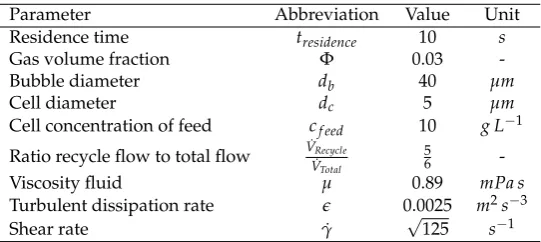
Rundzelle). To compare different simulations, a set of standard parameters (Table2) is introduced. 263
The parameters have been used for the simulations, unless other parameter settings are mentioned. 264
The turbulence dissipation rate and the shear rate are chosen in a range as observed at the inlet of 265
the investigated flotation tank. The residence time is chosen arbitrarily, whereas the other standard 266
parameters are set to reasonable values. 267
Table 2.Standard parameters for simulations
Parameter Abbreviation Value Unit
Residence time tresidence 10 s
Gas volume fraction Φ 0.03
-Bubble diameter db 40 µm
Cell diameter dc 5 µm
Cell concentration of feed cf eed 10 g L−1
Ratio recycle flow to total flow V˙Recycle
˙
VTotal
5
6
-Viscosity fluid µ 0.89 mPa s
Turbulent dissipation rate e 0.0025 m2s−3
Shear rate γ˙
√
125 s−1
4.1. Comparison of the different aggregation models 268
In this section the heteroaggregation models are compared, whereby a plug flow is assumed, i.e. 269
flow conditions stay constant during the simulation. For constant flow conditions, the modelAveraged 270
has an analytical solution which is derived in the AppendixA. The analytical solution includes the 271
dimensionless groupsΠ1andΠ3
272
Π1 =
1 4·
cc,0·d2c,0
cb,0·d2b,0
(33)
0
0.2
0.4
0.6
0.8
Aggregation number -
&
30
0.2
0.4
0.6
0.8
1
Separation efficiency
Averaged Not Averaged Poly.Cells Poly.Bubbles Clustering
Clustering Averaged
(a) Separation efficiency depending on aggregation number atΠ1=0.099
0.05
0.1
0.15
0.2
Maximal surface coverage -
&
10
0.2
0.4
0.6
0.8
1
Separation efficiency
Averaged Not Averaged Poly.Cells Poly.Bubbles Clustering
Clustering Averaged
(b)Separation efficiency depending on maximal surface coverage atΠ3=0.971
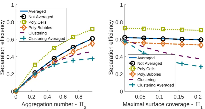
Figure 2.Comparison between the different aggregation models (Poly.Cells:σrel(dc) =0.25;Poly.Bubbles: σrel(db) =0.25)
wherecc,0is the initial number concentration of cells,cb,0the initial bubble concentration,tresidence
273
the residence time in the contact zone, andβunloaded(dc,0,db,0)the aggregation kernel for cells and
274
unloaded bubbles.Π1is the fraction of the initial bubble surface area that can be theoretically occupied
275
by the cells assuming the most favorable aggregation conditions. A high aggregation numberΠ3
276
corresponds to frequent aggregation. For the standard parameter settingsΠ1=0.099 andΠ3=0.971.
277
The separation efficiencies of the heteroaggregation models are calculated with Equation (16) 278
and plotted over the two dimensionless groupsΠ1 andΠ3(Figure2). IfΠ3 = 0, the efficiency is
279
zero, because no aggregation can occur. Then, the efficiency increases with an increasing aggregation 280
number, since a high aggregation number results from favorable collision conditions. A highΠ1
281
results from a high ratio between the projected surface of all cells and the surface of all bubbles. Thus, 282
the efficiency decreases with an increasingΠ1. To calculate the separation efficiency as described in
283
Equation (16),Π1has to be chosenΠ1>0. For very small values ofΠ1, the separation efficiencies of
284
the different models show already differences. 285
No difference between the modelsAveragedandNot Averagedcan be observed in the entire range 286
of the dimensionless groupsΠ1andΠ3. It can be observed, that the loading of the bubbles for the
287
modelAveragedapproximately equals to the mean loading of bubbles for the modelNot Averaged(data 288
not shown). 289
The cell size distribution of microorganisms can be described by a gamma distribution [42], which 290
allows setting the mean value and the standard deviation and guarantees positive diameters. Thus, in 291
the modelPoly.Cellsthe initial cell size distribution is set to a gamma distribution. In our model, the 292
mean diameter is equal to the standard parameterdc,mean=5µmand the relative standard deviation
293
σrel = dc,meanσ is 0.25. The efficiency of the modelPoly.Cellsis higher than the efficiency of the model
294
Averagedin the entire range ofΠ3andΠ1, which is discussed in detail in the next section. Additionally,
295
the difference between the two models tends to increase with higher relative standard deviations 296
is assumed to be a gamma distribution with the mean diameter equal to the standard parameter 298
db,mean=40µmandσrel =0.25. The efficiency of the model with polydisperse bubbles is lower than
299
the efficiency of the modelAveragedfor the entire ranges of the dimensionless groupsΠ1andΠ3.
300
A possible explanation for this observation is, that most of the bubbles’ volume is represented in 301
larger bubble sizes, since the volume of a single bubble is proportional to the bubble diameter cubed. 302
However, large bubbles are less efficient in floating cells than small bubbles [12]. The ratio between the 303
surface and the volume of a bubble decreases with an increasing bubble diameter. This results in an 304
increased maximal surface coverage and a decreased flotation efficiency for larger bubbles. 305
The lower the standard deviations of the modelsPoly.CellsandPoly.Bubbles, the more similar are 306
the results compared to the modelAveraged(data not shown). 307
The separation efficiencies of the modelsClusteringandClustering Averagedare lower than the 308
separation efficiencies of the modelAveragedin the whole range ofΠ1andΠ3. Additionally, the model
309
Clustering Averagedyields lower separation efficiencies than the modelClustering. This could be caused 310
by an overestimation of the cluster formation for the modelClustering Averaged. In general, clustering 311
reduces the efficiency because the formation of clusters with multiple bubbles reduces the available 312
surface area of bubbles. Therefore, the frequency of the attachment of cells decreases. 313
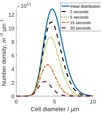
4.1.1. Influence of the cell size distribution 314
To investigate the influence of a distributed cell diameter on the efficiency of the flotation 315
process, the number density distribution of unbounded cells is computed at different simulation times 316
(see Figure3) for the modelPoly.Cells. The applied relative standard deviation isσrel =0.25. Each
317
distribution below the initial distribution signifies a subsequent simulation time. Due to aggregation 318
with bubbles the number density distribution of free cells decreases with an increasing simulation 319
time. Furthermore, the number density of bigger cells decreases significantly faster than the number 320
densities of smaller cells. Since the mass of a single cell is proportional to the cell diameter cubed, 321
most of the mass of the cells is represented in larger cell sizes and aggregates quite fast. Therefore, the 322
efficiency increases using a gamma distribution for the cell diameter as can be observed in Figure2. 323
324
0
5
10
Cell diameter / µm
0
2
4
6
8
10
12
Number density, m
-3
µm
-1
#
10
11 Initial distribution 2 seconds 5 seconds 15 seconds 30 seconds4.1.2. Mechanisms leading to the formation of clusters 325
To detect the main effects influencing the formation of aggregates with multiple bubbles, the 326
influence of the flow conditions are investigated. The turbulent dissipation rateeand the shear rate
327 ˙
γare varied, while the dimensionless groupsΠ1andΠ3are kept constant (see Figure4a). Thus,
328
the aggregation mechanisms due to laminar shear and turbulent motion are varied. The turbulent 329
dissipation rateeand the shear rate ˙γare plotted depending on their standard parameterseStand ˙γSt.
330
SinceΠ1andΠ3are kept constant, the efficiency for the analytical model does not change over the
331
entire parameter range. In absence of shear and turbulencee=γ˙ =0, the separation efficiencies of
332
the modelsClusteringandAveragedare equal. With increasingeand ˙γ, the efficiency of the clustering
333
model decreases significantly. Figure4billustrates two number density distributions of clusters with 334
a certain bubble number at a residence time of 10 seconds. Therein, the green dots represent the 335
simulation of the modelClusteringwith no turbulence and no shear, i.e.,e/eSt =0 and ˙γ/ ˙γSt =0. The
336
orange dots represent the simulation with the standard parameters fore= eStand ˙γ =γ˙St. In the
337
case of no turbulence and no shear, it can be observed, that there are almost no aggregates consisting 338
of more than one bubble. The aggregation mechanism is only due to sedimentation. This aggregation 339
mechanism does not seem to cause clustering of aggregates with multiple bubbles significantly. On the 340
contrary, for high turbulence and high shear, aggregates consisting of several bubbles are formed. This 341
lowers the efficiency, since the available surface of bubbles decreases, where cells can aggregate. It can 342
be deduced, that shear and turbulence cause clustering. 343
0
0.5
1
0
=
0
St;
.
_
=
.
_
St0
0.2
0.4
0.6
0.8
1
Separation efficiency
Analytical Model Clustering Model
(a)Separation efficiency.
5
10
15
Number of bubbles per cluster
0
2
4
6
8
Number density distribution / m
-3
#
10
11No turbulence and no shear Turbulence and shear
(b)Number density distribution of clusters for the two extreme cases.
Figure 4.Investigation on effect of variation of turbulent eddy dissipation and shear rate for constant Π1andΠ3on cluster formation.
4.1.3. Scope of aggregation models 344
The properties and scopes for the different aggregation models are illustrated in Table3. Due to 345
comparable modeling approaches, the separation efficiencies for the aggregation models are identical 346
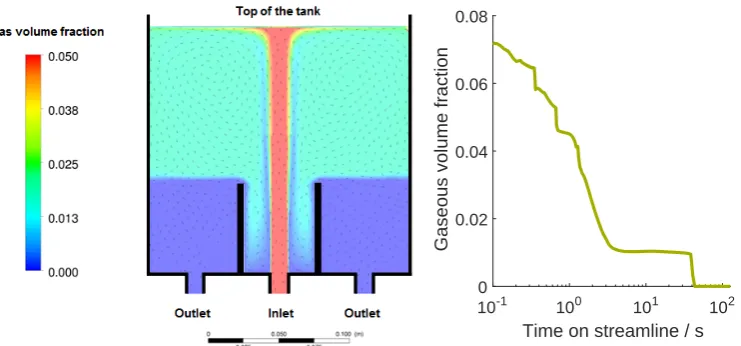
for the case of monodisperse cells and bubbles and without turbulence and laminar shear (data not 347
(a)Gas volume fraction and velocity directions of fluid
10-1 100 101 102
Time on streamline / s
0 0.02 0.04 0.06 0.08
Gaseous volume fraction
(b)Evolution of the gas volume fraction of a single streamline
Figure 5.Process conditions of the investigated flotation tank
of the aggregation model but also the simulation time. If cell and bubble sizes show small standard 349
deviations, the modelsAveraged,Not Averaged,ClusteringandClustering Averagedcan be used for model 350
based optimization. Generally, the modelAveragedshould be preferred to the modelNot Averaged 351
for determining efficient plant configurations and process conditions, since it requires much less 352
computational and modeling efforts and yields the same results. Since polydispersity of cells and 353
bubbles influence the efficiency, cell and bubble diameter distributions should be considered for quite 354
high standard deviations by using the modelsPoly.CellsorPoly.Bubbles. Turbulence and laminar shear 355
cause the formation of clusters, which lowers the flotation efficiency. Due to the low simulation time 356
and complexity, the modelClustering Averagedmay be preferred to the modelClusteringfor direct 357
coupling to CFD, if turbulence and laminar shear are sufficiently high to require consideration of cluste 358
formation. The two clustering models are also applicable, if the cells exist as aggregates which are 359
bigger than the microbubbles. 360
4.2. Lagrangian approach 361
In this section, the aggregation models are coupled with Euler/Euler CFD simulations for the 362
commercially available DAF system from Enviplan (AQUATECTOR®Microfloat®) with a flow rate 363
of 75 l/h. The geometry and the distribution of the gas volume fraction of the tank are illustrated in 364
Figure5a. From the inlet to the top of the tank, the gas volume fraction is quite high in a narrow area, 365
which is the main stream of the tank. At the top of the tank, most of the bubbles remain in the foam. 366
The other areas of the tank do not have such a high gas volume fraction. Close to the outlet,Φis zero. 367
Exemplarily, the heteroaggregation on one streamline of the DAF tank is investigated in detail. 368
4.2.1. Gas volume fraction 369
The investigated streamline has a residence time of about 140 seconds. The development of the gas 370
volume fraction is illustrated in Figure5b. Examining the coordinates of the CFD data (not illustrated 371
here) shows, that the top of the tank is reached in about 1.5 seconds. After approximately 3 seconds 372
the streamline leaves the top of the tank and flows to the outlet. During this time,Φdrops from 0.07 to 373
0.01. At the lower part of the tank,Φis zero. With the assumption that bubble-cell aggregates behave 374
like unloaded bubbles, all cells, which are attached to bubbles, float. Only the unbound cells remaining 375
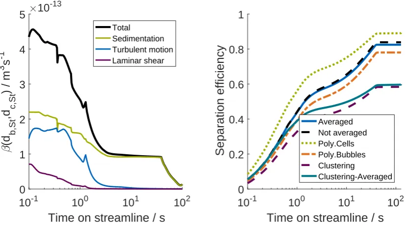
4.2.2. Aggregation mechanisms 377
The aggregation kernelβ(db,St,dc,St)of unloaded bubbles and free cells is illustrated as a function
378
of time on the investigated streamline in Figure6a. 379
10
-110
010
110
2Time on streamline / s
0
1
2
3
4
5
-(d
b,St
,d
c,St
) / m
3
s
-1
#
10
-13Total
Sedimentation Turbulent motion Laminar shear
(a)Importance of aggregation mechanisms on a single streamline
10
-110
010
110
2Time on streamline / s
0
0.2
0.4
0.6
0.8
1
Separation efficiency
Averaged Not averaged Poly.Cells Poly.Bubbles Clustering
Clustering-Averaged
(b) Separation efficiencies for different aggregation models
Figure 6. Aggregation mechanisms on a single streamline and resulting separation efficiencies for different aggregation models for this streamline
The total aggregation kernel for the streamline is high in the first 3 seconds. Then it stays nearly 380
constant until approximately 40 seconds. Between 40 and 90 seconds, βdecreases. Then, close to
381
the outlet,βincreases again. During the first 2 seconds the aggregation due to turbulent motion and
382
laminar shear has a noticeable influence on the total aggregation kernel. Afterwards, sedimentation is 383
the only important aggregation mechanism. The aggregation kernel depends on the hydrodynamic 384
encounter efficiency, which depends on the gas volume fraction. Therefore, when the gas volume 385
fraction decreases after 40 seconds, the aggregation kernel decreases as well. The last 50 seconds (not 386
shown here), the aggregation kernel increases again, since the fluid velocity increases in the region of 387
the outlet. However, this part is not important for the aggregation process, since in this region, the gas 388
volume fraction is already zero, and no aggregation between bubbles and cells can occur. The results 389
for other streamlines (data not shown) are similar. 390
4.2.3. Comparison of different aggregation models 391
In this section, the separation efficiencies of the investigated streamline are calculated for different 392
aggregation models. The relative standard deviations of the bubble diameter and the cell diameter 393
for the modelsPoly.CellsandPoly.Cellsareσrel =0.25. In Figure6b, the separation efficiencies of the
394
investigated streamline are illustrated. The efficiency for the modelAveragedincreases quickly in the 395
first 3 seconds and reaches an efficiency of about 0.6. Then, the efficency levels off until at a residence 396
time of approximately 40 seconds the efficiency reaches about 0.8. The trend of the flotation efficiency 397
is the same for all aggregation models. The fast aggregation process during the first few seconds can 398
be explained by the high gas volume fraction and the high aggregation kernel during this time. Then 399
decrease. At a residence time of 40 seconds, the gas volume fraction drops to zero and there is no 401
aggregation any longer. The efficiencies of the modelsNot AveragedandAveragedare comparable. The 402
efficiency of the model with polydisperse bubbles is smaller than the efficiency of the modelAveraged, 403
since most of the bubbles’ volume is distributed for larger bubble sizes in the used gamma distribution 404
for the bubbles. Large bubbles result in highΠ1and are less efficient in floating cells. In contrast, the
405
efficiency for the modelPoly.Cellsis higher than the efficiency for the modelAveraged. This is caused 406
by the fact, that most of the cell mass is distributed for larger cells. With an increasing cell diameter, 407
the aggregation kernel increases andΠ1decreases. Both effects lead to an increased flotation efficiency.
408
The formation of clusters reduces the available surface area of bubbles and reduces the frequency 409
of the attachment of cells. Therefore, the clustering models show lower separation efficiencies. The 410
results for the other streamlines (data not shown) are similar. 411
5. Conclusion 412
Down-stream separation of microorganisms using DAF or microflotation lacks applicable rigorous 413
modeling approaches for the heteroaggregation between microorganisms and microbubbles. Therefore, 414
different mechanistic aggregation models were introduced in the present study. Three models were 415
adapted from literature and three new were derived. The models allowed representing the distributed 416
character of bubble and cell sizes as well as the formation of clusters consisting of several bubbles and 417
cells. To determine the impact of the model assumptions, the modeling approaches were compared and 418
classified for their range of applicability. Additionally, the different aggregation models were coupled to 419
CFD data of a commercially available DAF system (Enviplan: AQUATECTOR®Microfloat®Rundzelle). 420
From model comparison it can be deduced, that turbulence and laminar shear form aggregates 421
consisting of several bubbles, whereas differential sedimentation only forms aggregates consisting of 422
a single bubble and multiple cells. The formation of aggregates with several bubbles decreases the 423
available surface, at which cells can aggregate. This lowers the separation efficiency. Additionally, 424
model comparisons show that bubble and cell size distributions can influence the separation efficiency 425
significantly and should be considered to determine efficient plant configurations and operating 426
conditions. 427
Once a suitable aggregation model has been selected from the discussed options, the flotation 428
process can be optimized computationally for separating the microorganisms. In this study the 429
encounter efficiency due to attractive and repulsive forces PA,0 was assumed to be unity. In an
430
extension to this paper,PA,0should be determined as described in the modeling section. This requires
431
detailed knowledge about the process conditions or experimental data. CFD data suggest, that the 432
classical two zone model is not accurate since fluid dynamics are highly heterogeneous in the flotation 433
tank. Thus, the aggregation models should be combined with the proposed Lagrangian approach 434
or directly coupled to CFD of the flotation process to determine efficient plant configurations and 435
process conditions. Direct coupling to CFD can be easily performed with the new developed averaged 436
approaches. 437
Author Contributions:S.R. provided the research idea; S.S, C.K., S.R., J.H. and H.B. conceptualized the work; 438
S.S. wrote the initial draft of the article and performed the PBM simulations; C.K. and H.B. supervised S.S.; J.H. 439
performed the CFD simulations; S.S, C.K., S.R., J.H. and H.B. discussed and interpreted the results and wrote the 440
final paper. 441
Funding:The authors thank BASF SE for the financial support for this work. 442
Acknowledgments:We thank Dr. Christian Riedele and Susanne Gulden for stimulating discussions. 443
Conflicts of Interest:The authors declare no conflict of interest. 444
Appendix A. ModelAveraged- Algebraic solution for two zone model 445
Aggregation equation 447
The general equation for aggregation for the modelAveragedis 448
dcc
dt =−β(dc,0,db)·cc·cb. (A1) Collision efficiency due to surface coverage
449
The total surface areaabof all bubbles per unit volume can be obtained by multiplying the surface
450
area of a single bubble with the bubble number concentration 451
ab =π·d2b·cb. (A2)
The total projected surface areaacof cells bound to bubbles per unit volume is
452
ac= π
4 ·d
2
c,0·(cc,0−cc), (A3)
The collision efficiency due to surface coverage is assumed to be proportional to the fraction of the 453
non-occupied surface area of the bubbles. 454
PA,S =
ab−ac
ab
(A4)
= 1−
π
4 ·d2c,0·(cc,0−cc) π·d2b·cb
(A5)
= 1− cc,0·d
2
c,0
4·cb,0·d2b
·
1− cc cc,0
. (A6)
Non-dimensionalization 455
First of all, the following non-dimensional variables are useful 456
˜
cc = cc
cc,0 (A7)
˜ cb =
cb
cb,0
(A8)
˜ db =
db
db,0
, (A9)
Substituting these non-dimensional variables into the efficiency due to surface coverage yields 457
PA,surface=1− Π1
˜ cbd˜2b
(1−c˜c). (A10)
PA,surface=1−
cc,0·d2c,0
4·d2
b·cb
·
1− cc cc,0
=1− cc,0·d
2
c,0
4·d2b,0·cb,0
·1−c˜c ˜ cb·d˜2b
=1− Π1 ˜ cbd˜2b
(1−c˜c), (A11)
whereΠ1is a dimensionless group.Π1can be expressed as:
Π1= 1
4·
cc,0·d2c,0
cb,0·d2b,0
. (A12)
Using 459
β(dc,0,db) =PA,sur f ace·K(dc,0,db), (A13)
the equation,which describes the general aggregation equation, can be transformed as follows: 460
dcc
dt =−PA,sur f ace·K(dc,0,db)·cc·cb (A14)
⇔d ˜cc
dt =− 1−
Π1
˜ cbd˜2b
(1−c˜c) !
·K
dc,0
db,0
·db,0,db,0·d˜b
·cb,0·c˜c·c˜b. (A15)
Implementing the dimensionless timeτ, the ratio of diameters of cells and bubbles Π2 and the
461
normalized aggregation frequency ˜K 462
τ = t·K(db,0·Π2,db,0)·cb,0 (A16)
Π2 =
dc,0
db,0
(A17)
˜
K = K(db,0·Π2,db,0·d˜b) K(db,0·Π2,db,0)
(A18)
one can transform the general aggregation equation 463
d ˜cc
dτ =− 1−
Π1
˜ cb·d˜2b
(1−c˜c) !
·K˜·c˜c·c˜b. (A19)
A dimensionless groupΠ3can be obtained - the aggregation number
464
Π3 = tresidence·K(db,0·Π2,db,0)·cb,0. (A20)
Analytical solution 465
Neglecting bubble coalescence, the concentration and diameter of the bubbles stay constant. 466
Furthermore, it is assumed that the aggregates have the diameter of a single bubble. Therefore 467
˜
cb(τ) =1 and ˜db(τ) =1, which leads to ˜K=1. The equation describing aggregation can be simplified
468 to: 469
d ˜cc
dτ =−(1−Π1·(1−c˜c))·c˜c. (A21)
By analytically integrating this differential equation fromτ = 0 toτ = Π3(t = tresidence), the cell
470
concentration at the end of the contact zone ˜cc,outcan be calculated as:
471
˜
cc,out= 1
−Π1
exp(Π3·(1−Π1))−Π1
. (A22)
Appendix B. Encounter efficiency due to surface coverage for clustering 472
To consider the reduction of the encounter efficiency due to surface coverage in the models 473
the cells of a cluster are uniformly distributed on the surface of all bubbles of the cluster. Moreover, 475
the clusters are packed densely. An attachment between two clusters can only occur if a cell of the 476
exposable surface area of a cluster collides with a bubble of the exposable surface area of the other 477
cluster or vice versa. Since bubble coalescence and aggregation is negligible [12], the aggregation 478
between bubbles is assumed to be impossible. Furthermore, the coagulation of cells is neglected. 479
Otherwise flocks would be formed and microflotation would not be necessary. With the assumption 480
that clusters are densely packed, the volume of a cluster consisting ofibubbles and jcells can be 481
calculated as the sum of the volume of the consisting bubbles and cells 482
Vi,j =i·Vb+j·Vc= 1
6 ·π
i·d3b+j·d3c
. (A23)
Additionally, the cluster volume can be described as 483
Vi,j =
1 6·π·d
3
i,j, (A24)
wheredi,jis the cluster’s equivalent diameter. Setting Equation (A23) equal to Equation (A24),di,jcan
484
be expressed as 485
di,j=
i·d3b+j·d3c 13
. (A25)
The exposed surface area of a cluster withibubbles andjcellsAexposed(i,j)is expressed as
486
Aexposed(i,j) =π·d2i,j=π·
i·d3b+j·d3c 23
. (A26)
The sum of the surface area of all bubbles of a cluster withibubblesAb,sur f ace(i,j)is calculated as
487
Ab,sur f ace(i,j) =i·π·d2b. (A27)
The sum of the projected surface area ofjcells of a clusterAc,proj(i,j)is expressed as
488
Ac,proj(i,j) =j· π
4 ·d
2
c. (A28)
Assuming that the cells of a cluster are uniformly distributed on the surface of all bubbles of the cluster, 489
the ratio of the exposed cluster surface which is occupied by cellsRp(i,j)is calculated as
490
Rp(i,j) =
Ac,proj(i,j)
Ab,sur f ace(i,j)
= j·d
2
c
i·4·d2
b
. (A29)
KnowingRp(i,j)the ratio of the exposable cluster surface which is occupied by bubblesRb(i,j)can be
491
expressed by 492
Rb(i,j) =1−Rp(i,j). (A30)
References 493
1. Christenson, L.; Sims, R. Production and harvesting of microalgae for wastewater treatment, biofuels, and 494
bioproducts. Biotechnology advances2011,29, 686–702. 495
2. Sarris, D.; Papanikolaou, S. Biotechnological production of ethanol: Biochemistry, processes and 496
technologies. Engineering in Life Sciences2016,16, 307–329. 497
3. Chisti, Y. Biodiesel from microalgae. Biotechnology advances2007,25, 294–306. 498
4. Larkum, A.W.; Ross, I.L.; Kruse, O.; Hankamer, B. Selection, breeding and engineering of microalgae for 499
bioenergy and biofuel production.Trends in biotechnology2012,30, 198–205. 500
5. Grima, E.M.; Belarbi, E.H.; Fernández, F.A.; Medina, A.R.; Chisti, Y. Recovery of microalgal biomass and 501
6. Barros, A.I.; Gonçalves, A.L.; Simões, M.; Pires, J.C. Harvesting techniques applied to microalgae: A review. 503
Renewable and Sustainable Energy Reviews2015,41, 1489–1500. 504
7. Soetaert, W.; Vandamme, E.J.Industrial biotechnology: sustainable growth and economic success; John Wiley & 505
Sons, 2010. 506
8. Ndikubwimana, T.; Chang, J.; Xiao, Z.; Shao, W.; Zeng, X.; Ng, I.S.; Lu, Y. Flotation: A promising microalgae 507
harvesting and dewatering technology for biofuels production. Biotechnology journal2016,11, 315–326. 508
9. Hanotu, J.; Bandulasena, H.; Zimmerman, W.B. Microflotation performance for algal separation. 509
Biotechnology and bioengineering2012,109, 1663–1673. 510
10. Hanotu, J.; Karunakaran, E.; Bandulasena, H.; Biggs, C.; Zimmerman, W.B. Harvesting and dewatering 511
yeast by microflotation.Biochemical Engineering Journal2014,82, 174–182. 512
11. Shawwa, A.R.; Smith, D.W. Dissolved air flotation model for drinking water treatment. Canadian Journal of 513
Civil Engineering2000,27, 373–382. 514
12. Edzwald, J.K. Dissolved air flotation and me. Water Research2010,44, 2077–2106. 515
13. Fukushi, K.; Tambo, N.; Matsui, Y. A Kinetic-Model for Dissolved Air Flotation in Water and Waster-Water 516
Treatment.Water Science and Technology1995,31, 37–47. International Specialised Conference on Flotation 517
Processes in Water and Sludge Treatment, Orlando. 518
14. Leppinen, D.; Dalziel, S. Bubble size distribution in dissolved air flotation tanks.Journal of Water Supply 519
Research and Technology - AQUA2004,53, 531–543. 520
15. Liers, S.; Baeyens, J.; Mochtar, I. Modeling dissolved air flotation. Water Environment Research1996, 521
68, 1061–1075. 522
16. Kwak, D.H.; Yoo, S.J.; Lee, E.J.; Lee, J.W. Evaluation on simultaneous removal of particles and off-flavors 523
using population balance for application of powdered activated carbon in dissolved air flotation process. 524
Water Science and Technology2010,61, 323–330. 525
17. Jung, H.; Lee, J.; Choi, D.; Kim, S.; Kwak, D. Flotation efficiency of activated sludge flocs using population 526
balance model in dissolved air flotation. Korean Journal of Chemical Engineering2006,23, 271–278. 527
18. Laamanen, C.A.; Ross, G.M.; Scott, J.A. Flotation harvesting of microalgae. Renewable and Sustainable 528
Energy Reviews2016,58, 75–86. 529
19. Zhang, X.; Wang, L.; Sommerfeld, M.; Hu, Q. Harvesting microalgal biomass using magnesium 530
coagulation-dissolved air flotation. Biomass and Bioenergy2016,93, 43–49. 531
20. Zhang, X.; Hewson, J.C.; Amendola, P.; Reynoso, M.; Sommerfeld, M.; Chen, Y.; Hu, Q. Critical evaluation 532
and modeling of algal harvesting using dissolved air flotation. Biotechnology and Bioengineering2014, 533
111, 2477–2485. 534
21. Leppinen, D.; Dalziel, S.; Linden, P. Modelling the global efficiency of dissolved air flotation. Water Science 535
and Technology2001,43, 159–166. 4th International Conference on Dissolved Air Flotation in Water and 536
Waste Water Treatment, Helsinki, Finland. 537
22. Kwak, D.H.; Jung, H.J.; Kwon, S.B.; Lee, E.J.; Won, C.H.; Lee, J.W.; Yoo, S.J. Rise velocity verification of 538
bubble-floc agglomerates using population balance in the DAF process. Journal of Water Supply Research 539
and Technology - AQUA2009,58, 85–94. 540
23. Matsui, Y.; Fukushi, K.; Tambo, N. Modeling, simulation and operational parameters of dissolved air 541
flotation. Journal of Water Services Research and Technology - AQUA1998,47, 9–20. 542
24. Lakghomi, B.; Lawryshyn, Y.; Hofmann, R. A model of particle removal in a dissolved air flotation tank: 543
Importance of stratified flow and bubble size. Water Research2015,68, 262–272. 544
25. Kostoglou, M.; Karapantsios, T.D.; Matis, K.A. CFD model for the design of large scale flotation tanks for 545
water and wastewater treatment. Industrial & Engineering Chemistry Research2007,46, 6590–6599. 546
26. Edzwald, J.K. Principles and applications of dissolved air flotation. Water Science and Technology1995, 547
31, 1–23. International Specialised Conference on Flotation Processes in Water and Sludge Treatment, 548
Orlando, FL, Apr 26-28, 1994. 549
27. Saffman, P.; Turner, J. On the collision of drops in turbulent clouds. Journal of Fluid Mechanics1956,1, 16–30. 550
28. Meyer, C.; Deglon, D. Particle collision modeling - A review.Minerals Engineering2011,24, 719 – 730. 551
29. Pedocchi, F.; Piedra-Cueva, I. Camp and Stein’s Velocity Gradient Formalization.Journal of Environmental 552
Engineering2005,131, 1369–1376. 553
30. von Smoluchowski, M. Versuch einer mathematischen Theorie der Koagulationskinetik kolloider Lösungen. 554
31. Nguyen, A.; Ralston, J.; Schulze, H. On modelling of bubble-particle attachment probability in flotation. 556
International Journal of Mineral Processing1998,53, 225–249. 557
32. Nguyen, A. Hydrodynamics of liquid flows around air bubbles in flotation: a review. International Journal 558
of Mineral Processing1999,56, 165–205. 559
33. Sasic, S.; Sibaki, E.K.; Strom, H. Direct numerical simulation of a hydrodynamic interaction between 560
settling particles and rising microbubbles. European Journal of Mechanics B - Fluids2014, 43, 65–75. 561
doi:10.1016/j.euromechflu.2013.07.003. 562
34. Dai, Z.; Fornasiero, D.; Ralston, J. Particle-bubble collision models - a review. Advances in Colloid and 563
Interface Science2000,85, 231 – 256. 564
35. Rollié, S.; Briesen, H.; Sundmacher, K. Discrete bivariate population balance modelling of heteroaggregation 565
processes.Journal of Colloid and Interface Science2009,336, 551–564. 566
36. Ren, Z.; Harshe, Y.M.; Lattuada, M. Influence of the Potential Well on the Breakage Rate of Colloidal 567
Aggregates in Simple Shear and Uniaxial Extensional Flows.Langmuir2015,31, 5712–5721. 568
37. Sun, W.; Zeng, Q.; Yu, A. Calculation of Noncontact Forces between Silica Nanospheres. Langmuir2013, 569
29, 2175–2184. 570
38. Rudolph, M.; Peuker, U.A. Hydrophobicity of Minerals Determined by Atomic Force Microscopy - A Tool 571
for Flotation Research.Chemie Ingenieur Technik2014,86, 865–873. 572
39. Ta, C.; Beckley, J.; Eades, A. A multiphase CFD model of DAF process. Water Science and Technology2001, 573
43, 153–157. 4th International Conference on Dissolved Air Flotation in Water and Waste Water Treatment. 574
40. Tomiyama, A.; Takamasa, T.Ansys 16.2.3; Interphase Exchange Coefficients: Tomiyama et al. Model (17.5.6.1.5.). 575
41. Kumar, J.; Peglow, M.; Warnecke, G.; Heinrich, S.; Morl, L. Improved accuracy and convergence of 576
discretized population balance for aggregation: The cell average technique.Chemical Engineering Science 577
2006,61, 3327–3342. 578
42. Iyer-Biswas, S.; Crooks, G.E.; Scherer, N.F.; Dinner, A.R. Universality in stochastic exponential growth. 579