An Implicitly Directly Additive Demand System: Estimates for Australia

Menzies Building

PO Box 11E, Monash University

Wellington Road

CLAYTON Vic 3800 AUSTRALIA

Telephone:

from overseas:

(03) 9905 2398, (03) 9905 5112 61 3 9905 5112 or 61 3 9905 2398

Fax:

(03) 9905 2426 61 3 9905 2426

e-mail

[email protected]

web site http://www.monash.edu.au/policy/

Paper presented to the Third General Equilibrium Modeling Conference Wilfred Laurier University, WATERLOO, Ontario 24-25 October 1992

AN IMPLICITLY DIRECTLY

ADDITIVE DEMAND SYSTEM:

ESTIMATES FOR AUSTRALIA

by

Maureen T. RIMMER Alan A. POWELL

Industry Commission

and

Monash University

Monash University

Preliminary Working Paper No. OP–73 October 1992

reissued August 2001

ISSN 1 031 9034 ISBN 0 7326 1527 5

The Centre of Policy Studies (CoPS) is a research centre at Monash University

devoted to quantitative analysis of issues relevant to Australian economic policy.

C

ENTRE

of

P

OLICY

S

TUDIES

and

the

I

MPACT

The problem of endowing large applied general equilibrium

models with numerical values for parameters is formidable. For

example, a complete set of own- and cross-price elasticities of

demand for the

ORANI

model involves 228

2

≈

60 K items. Invoking

the minimal assumptions that demand is generated by utility

maxi-mization reduces the load to about 26 K Ñ obviously still a number

much too large for unrestrained econometric estimation.

To obtain demand systems estimates for a dozen or so generic

commodities at a top level of aggregation (categories like 'food',

'clothing and footwear', ...), typically Johansen's (1960) lead has

been followed, and directly additive preferences imposed upon the

underlying utility function. With the move beyond one-step

linearized solutions of the

ORANI

model, the functional form of the

demand system adopted becomes an issue. The most celebrated of

the additive-preference demand systems, Stone's (1954)

linear

expenditure system

(LES), has one drawback for empirical work;

namely, the constancy of marginal budget shares (MBSs) Ñ a liability

shared with the Rotterdam system (Barten, 1964, 1968; Theil,

1965, 1967). To get around this, Theil and Clements (1987) used

Holbrook Working's (1943) Engel specification in conjunction with

additive preferences; unfortunately both Working's formulation and

Deaton and Muellbauer's (1980) AIDS have the problem that, under

large changes in real incomes, budget shares can stray outside the

[0,1] interval. It was such behaviour that led Cooper and McLaren

(1987, 1988, 1991, forthcoming 1992) to invent MAIDS, a system

with better regularity properties. MAIDS, however, is not globally

compatible with any additive preference system.

i

1. Introduction 1

2. AIDADS Ñ A Generalization of Les 3

2.1 The new expenditure system 3

2.2 Substitution properties 5

2.3 Engel properties Ñ I 5

2.4 Differential form of AIDADS 6

2.5 Engel properties Ñ II 8

3. Strategy for Estimation 10

3.1 Estimating equation I Ñ non-stochastic part 10

3.2 Estimating equation II Ñ stochastics and error correction 15

3.3 Computation of ML Estimator 17

4. The Data 21

5. Results 22

5.1 Estimation in the levels 22

5.2 Estimation in the differences 23

5.3 Price and substitution elasticities 34

6. Concluding Remarks 34

ii

4.1 The Six Commodity Level of Disaggregation of Final

Consumption Expenditure 21

4.2 Details of Available Constant-Price Data 21

5.1 Maximum Likelihood Estimates of AIDADS fitted in the

Levels, Without Error Correction: Annual Australian Data,

1954-55 through 1988-89 24

5.2 Maximum Likelihood Estimates of AIDADS fitted in the

Levels, With Error Correction: Annual Australian Data,

1954-55 through 1988-89 24

5.3 Maximum Likelihood Estimates of AIDADS fitted in the

First Differences, Annual Australian Data, 1954-55

through 1988-89 25

5.4 Estimated Substitution Elasticities for AIDADS at Beginning

and End of Sample (from the Levels Estimation without

Error Correction) 25

5.5 Estimated Substitution Elasticities for AIDADS at Beginning

and End of Sample (from the Levels Estimation with Error

Correction) 31

5.6 Estimated Substitution Elasticities for AIDADS at Beginning

and End of Sample (from the First Differences Estimation) 31

5.7 Estimated Engel and Own and Cross-Price Elasticities

for the Mid 1950s 32

5.8 Estimated Engel and Own and Cross-Price Elasticities

iii

2.1(a) Engel curves which show globally constant unit elasticity

or which are irregular in certain regions 11

2.1(b) Engel Curve in the Linear Expenditure System for a necessity 11

2.1(c) Engel Curve in the Linear Expenditure system for a luxury 12

2.1(d) These Engel Curves for the AIDADS system were generated

by simulations using the framework shown in Figure 3.1 12

2.1(e) These Engel Curves for the AIDADS system were generated

by simulations using the framework shown in Figure 3.1 13

2.1(f) This Engel Curve for the AIDADS system was generated

by simulations using the framework shown in Figure 3.1 13

3.1 Flow chart for data/parameter transformations in

computation of the ML estimates 20

5.1 AIDADS fitted in the levels (without error correction) to

Australian data on budget shares, 1954-55 through 1988-89 26

5.2 AIDADS fitted in the levels (with error correction) to

Aust-ralian data on budget shares, 1954-55 through 1988-89 27

5.3 AIDADS fitted in the levels (with error correction) to Aust-ralian data on budget shares, 1954-55 through 1988-89

Ñ plot of equilibrium and actual values 28

5.4 AIDADS fitted in the differences (with error correction) to Australian data on budget shares, 1954-55 through 1988-89

Ñ plot of first differences of shares 29

5.5 AIDADS fitted in the differences (with error correction) to Australian data on budget shares, 1954-55 through 1988-89

E

STIMATES FOR

A

USTRALIA

*

by

Maureen T. RIMMER and Alan A. POWELL

Industry Commission

and Monash University

Monash University

1. Introduction

The problem of endowing large applied general equilibrium models with numerical values for parameters is nowhere more difficult than in the consumption side of the models. In the ORANI model of the Australian economy1_{, for instance, there are 228}

commodities recognized (114 input-output commodities, each with a locally made and an overseas variant). A complete set of own- and cross-price elasticities of demand hence involves 2282 ≈ 60 K items. Invoking the minimal assumption that demand is generated by maximization of a strictly quasi-concave utility function reduces the information load to about 26 K (i.e., 227 + (228_ÊÊ2 ) ). Obviously such a large number of elasticities could not be estimated econometrically from available data without the use of prior restrictions on functional form.

The traditional approach in applied GE work involves starting at some higher level of aggregation Ñ in the case of ORANI, with about a dozen generic commodities. Each of these is defined as a simple aggregate of a subset of the 114 input-output commodities. The latter in turn are seen as Armington (CES) aggregates of the domestically sourced and the foreign commodity of the same name. The elasticities of substitution between the domestic and the foreign variant of each input-output commodity are then estimated, where feasible, from time-series data (see, e.g., Alaouze (1977), Reinert and Shiells (1991), Reinert and Roland-Holst (forthcoming 1992)).

To obtain demand systems estimates for the dozen or so generic commodities (categories like 'food', 'clothing and footwear', ...), typically Johansen's (1960) lead has been followed, and directly additive preferences imposed upon the underlying utility function (e.g., TulpulŽ and Powell (1978)). The principal advantages of the additive preference postulate are two:

(1) it greatly reduces the number of parameters that have to be estimated. Whereas the 12 commodity system estimated under minimal assumptions involves

₍

12

2

)

= 66 substitution parameters, additive preferences when fitted

in the levels need involve no more than 12 (and only one, the so-called 'Frisch parameter' if fitted in the differences);

(2) at the high level of aggregation at which it is applied, additive preferences fits time-series data well, with little evidence of gross misspecification.

Disaggregation from the 12 or so commodities at the top level to the 100 or so input-output commodities presents serious challenges. Where econometric work can be done at a finer level of disaggregation, however, it is relatively straightforward to incorporate

* _{The authors would like to thank Russel Cooper, Eric Ghysels, Jill Harrison, Brett Inder and}

Keith McLaren for helpful suggestions.

new elasticities at the input-output level of disaggregation (Clements and Smith, 1983) provided that the utility function is nested so as to leave undisturbed its upper levels.2

With the move beyond one-step linearized solutions of the ORANI model, the functional form of the demand system adopted becomes an issue, even within the additive preference framework (at which we continue to work at the top level of aggregation).3 _{The most celebrated of the additive-preference demand systems, Stone's}

(1954) linear expenditure system (LES), has one drawback for empirical work; namely, the constancy of marginal budget shares (MBSs)4 _{Ñ a liability shared with the Rotterdam}

system (Barten, 1964, 1968; Theil, 1965, 1967). Holbrook Working (1943) provided a parsimonious yet empirically successful way of allowing marginal budget shares to respond to income levels; his is the Engel specification adopted within Deaton and Muellbauer's (1980) almost ideal demand system (AIDS). Theil and Clements (1987) used Working's specification in conjunction with additive preferences; unfortunately from the current perspective, their system is formulated and implemented only in the differentials. And in any event, Working's formulation (and AIDS) has the problem that, under large changes in real incomes, budget shares5 _{can stray outside the [0,1] interval.}

It was such irregular behaviour that led Cooper and McLaren (1987, 1988, 1991, 1992a) to modify the AIDS system to become MAIDS, a system with regular properties over a much wider subset of the price-expenditure space. MAIDS, however, is not globally compatible with any additive preference system.

What we hope to achieve in this paper is to specify, and to estimate, at the six-commodity level, an additive-preference demand system that is globally regular throughout that part of the the price-expenditure space in which the consumer is at least affluent enough to meet subsistence requirements and which allows MBSs to vary as a function of total real expenditure. Such an estimated system will be directly comparable (via its Frisch 'parameter') to other additive-preference systems currently in use in applied general equilibrium work, but will be more flexible in its treatment of Engel effects than the LES or Rotterdam models, and have better regularity properties than AIDS or other versions of Working's model. Our starting point is Hanoch (1975).

In Section 2 a special case of Hanoch's directly, but implicitly, additive-preference demand system is set out. In Section 3 the model is endowed with a stochastic dimension, and a strategy for its estimation is developed. Sections 4 and 5 respectively contain a brief description of the data, and a full account of the estimation results. A concluding perspective is offered in Section 6.

2. AIDADS Ñ A Generalization of LES

2 Failing the availability of disaggregated estimates, it is common practice to use a globally

additive preference specification, even though it is known that this is a serious misspecification of the demand structure at the detailed level.

3 When working with small displacements of an additive-preference demand system, only the

local values of the demand elasticities are relevant. To determine a complete set of the latter it is only necessary to know the local values of the expenditure elasticities, and of the Frisch 'parameter'.

4 _{Let xi stand for the quantity of i demanded, pi for its price, and M for total nominal}

expenditure. By the ith _{marginal budget share we mean pi}∂_xi/∂M.

5 By budget share or average budget share (in the notation of the previous footnote) we mean

2.1 The new expenditure system

The demand system now derived will be referred to as AIDADS (an implicitly directly additive demand system). Hanoch (1975) defines implicit direct additivity by the utility function:

(2.1.1)

Σ

i=1 n

Ê

U_i(x_i , u) = 1,

where {x₁, x₂, ... , x_n} is the consumption bundle, u is the level of utility, and the U_i are twice-differentiable monotonic functions satisfying appropriate concavity conditions. Using some intuition stemming from Cooper and McLaren's MAIDS and from the LES, we choose the U_i as follows:

(2.1.2) U_i =

[α_iÊ+Êβ_iÊG(u)]

Ê[1Ê+ÊG(u)] ln

(

Êx_iÊÐÊγ_i

ÊAÊeuÊÊ

)

= φi ln

(

Êx_iÊÐÊγ_i

ÊAÊeuÊÊ

)

,

(i = 1, 2, ..., n)

where G(u) is a positive, monotonic, twice-differentiable function, and the lower-case Greek letters are parameters, with

(2.1.3) 0 ≤ α_i , β_i ≤ 1;

Σ

i=1 n

Ê_α

i = 1 =

Σ

i=1 n

Ê_β

i .

Hanoch (1975) notes that the first-order conditions for minimizing the cost M of obtaining a given level of utility u are (2.1.1) and:

(2.1.4) λ∂U_i/ ∂x_i = p_i, (i = 1, 2, ..., n)

where λ is the Lagrange multiplier on (2.1.1) and {p₁, p₂, ... , p_n} is the set of commodity prices. In the case of our choice of the U_i, (2.1.4) becomes:

(2.1.5)

λÊ[

α

_iÊ+Êβ_iÊG(u)]

(

x_iÊÐÊγ_i

)Ê

[1Ê+ÊG(u)] = pi . (i = 1, 2, ..., n)

Hence

(2.1.6) λÐÊ1 p_iÊ(x_i Ð γ_i) = [

α

_i + β_i G(u)] / [1 + G(u)] .

(i = 1, 2, ..., n)

Using the budget identity

(2.1.7)

Σ

i=1 n

Ê

p_i x_i = M,

where M is total money expenditure (endogenous in this problem), by adding (2.1.6) across i and using (2.1.3), we obtain:

(2.1.8) λÊÐ1 (M Ð p′ γ) = 1,

(2.1.9) λ = (M Ð p′ γ) ,

where in (2.1.8) and (2.1.9) p'γ is shorthand for

∑

i=1 n

Ê p_iγ_{i . Back-substituting from}

(2.1.9) into (2.1.6), after rearrangement we obtain

(2.1.10a) p_iÊ(x_i Ð γ_i) =

φ

_i (M Ð p′ γ) , (i = 1, 2, ..., n)

where

φ

_{i was defined implicitly by (2.1.2) as}

(2.1.10b)

φ

_i =

[

α

_iÊ+Êβ_iÊG(u)]

[1Ê+ÊG(u)Ê]Ê . (i = 1, 2, ..., n)

For later use we note that φ_i may be interpreted as the share W°_i of discretionary expenditure on commodity i in total discretionary expenditure (M - p′γ).

In the form (2.1.10b) we see the direct connection between the LES and AIDADS; setting every

α

_i equal to the corresponding β_i causes

φ

_i to collapse to just β_i , which reduces (2.1.10a, b) to the LES. Note that the φ_is add over i to unity.

An alternative derivation of (2.1.10a) keeps total expenditure exogenous, not only in the final expenditure system, but also in the problem faced by the optimizing agent. Instead of minimizing M subject to a given u with preferences constrained by (2.1.1), maximize u subject to (2.1.1) and (2.1.7), by first constructing the Lagrangean:

(2.1.11) L = u + Λ













Σ

i=1 n

ÊU_iÊ(x_i,Êu)ÊÐÊ1 + χ (M Ð p′x) .

The first-order conditions are (2.1.1), (2.1.7) and

(2.1.12) _∂∂u

x_i + Λ













∂U_i

∂_xiÊÊÊ+ÊÊ

Σ

j=1 n

ÊÊ ∂U_j

∂uÊÊ ∂u

∂x_i = χ pi. (i = 1, 2, ..., n)

By taking the total differential of (2.1.1) it is apparent that6

(2.1.13) _∂∂u

x_i = Ð

∂U_i

∂x_i

/

Σ

k=1 n

∂U_k

∂u ; (i = 1, 2, ..., n)

that is, that the term multiplied by Λ in (2.1.12) vanishes identically. Substituting from (2.1.13) into (2.1.12) and using (2.1.2), we obtain

(2.1.14a)

∂U_i

∂x_i = Ð χ pi

Σ

k=1 n

∂U_k ∂u .

(2.1.14b) = φ_i / (x_i Ð γ_i) . (i = 1, 2, ..., n)

Clearing fractions and summing over i we obtain:

(2.1.15) χ = Ð













(MÊÐÊp′Êγ)Ê

Σ

k=1 n

ÊÊ ∂U_k

∂u

Ð1

Back substituting from (2.1.15) into (2.1.14a), we recover (2.1.10a).

2.2 Substitution properties

Hanoch (1975, p.400) notes that the substitution elasticities associated with implicit direct additivity are:

(2.2.1) σ_{i j} =

ÊÊÊÊÊÊÊÊa_i(x_i,Êu)Êa_j(x_j,Êu)ÊÊ

ÊÊ

∑

k=1 n

ÊakÊÊ(Êxk,Êu)ÊWkÊ ,

(i≠j, i ,j = 1, 2, ..., n)

where

(2.2.2) a_i(x_i, u) =

ÊÐÊ∂U_i/Ê∂x_iÊ

ÊÊx_iÊ∂2ÊU_i/Ê(∂x_iÊ∂x_iÊ)ÊÊÊ = (xi Ð γi)/xi

(i = 1, 2, ..., n)

and

(2.2.3) W_k = x_kp_k / Μ , (k = 1, 2, ..., n)

where in (2.2.3) we have assumed that the consumer behaves optimally (i.e., that (2.1.4) holds. The Ws are to be interpreted as budget shares. Substituting from (2.2.3) and (2.2.2) into (2.2.1), we obtain:

(2.2.4) σ_{i j} =

(x_iÊÐÊγ_i)Ê(x_jÊÐÊγ_j)Ê

x_iÊx_j

/

(MÊÐÊp′Êγ)Ê

MÊÊ . (i≠j, i ,j = 1, 2, ..., n)

These take exactly the same form as the partial substitution elasticities in the matching LES. If the γs are all positive (as is insisted upon in some interpretations of additive preferences), the σ_ij in LES and in AIDADS tend to unity as income grows very large.

At this point it is clear that AIDADS has exactly similar substitution properties to LES, but that the former has richer Engel possibilities. These come at the expense of an additional (nÐ1) parameters; namely, the (nÐ1) independent values of α_i.

2.3 Engel properties Ñ I

Not much further progress can be made without specifying a functional form for G. Here we keep the LES interpretation of γ as the subsistence bundle, and require as well that

(2.3.1a) lim

xÊ→Ê

∞

Ê u(x) =

∞

;

(2.3.1b) lim

xÊ→Ê

γ+

Ê u(x) = Ð

∞

;

(2.3.1c) lim

uÊ→Ê

∞

Ê G(u) =

∞

;

(2.3.1d) limÊ

uÊ→Ê

ÐÊ

∞

Ê

Ê G(u) =

0 .

(Above x is the bundle {x₁, x₂, ..., x_n}, and the notation x →

∞

implies that every

x

_i

grows without limit, while x →

γ

+ implies that each

x

_{i converges to its corresponding}

γ

_iÊfrom above.) G's monotonicity together with the bounds imposed on it above ensure that

φ

_i behaves logistically, remaining always in the [α_i, β_i] interval. It can be shown that if

α

_i < β_i, the logistic behaviour of

φ

_i implies that the lowest value of i's marginal budget share is

α

_i, occurring when total expenditure is just enough to cover purchase of the subsistence bundle

γ;

theupper asymptote of MBS_iÊ as expenditure grows without limit is β_i. If, on the other hand,

α

_i > β_i, the largest value of i's marginal budget share is

α

_i, occurring at the subsistence expenditure level; its asymptote as expenditure grows indefinitely large and lowest value is β_i.

The Engel elasticities in AIDADS are:

(2.3.2)

ε

_i

=

φ

_iÊÊÊM

ÊÊÊp_iÊγ_iÊÊ+ÊÊ

φ

_iÊÊ(MÊÊÊÐÊÊp′Êγ)ÊÊ +

[

∂φ

_i

/∂

Μ

]

ÊΜÊÊ(MÊÊÊÐÊp′Êγ) ÊÊÊp_iÊγ_iÊÊ+ÊÊ

φ

_iÊÊ(MÊÊÊÐÊÊp′Êγ)ÊÊ

=

φ

iÊÊÊM

ÊÊÊp_iÊγ_iÊÊ+ÊÊ

φ

_iÊÊ(MÊÊÊÐÊÊp′Êγ)ÊÊ +

[

∂φ

_i

/∂

u

]

Ê

[

∂

u

/∂

Μ

]

ÊΜÊÊ(MÊÊÊÐÊÊp′Êγ) ÊÊÊp_iÊγ_iÊÊ+ÊÊ

φ

_iÊÊ(MÊÊÊÐÊÊp′Êγ)ÊÊ .

(i = 1, 2, ..., n)

Further progress cannot be made without specifying a functional form for G. The simplest G(¥) satisfying (2.3.1c&d) is:

(2.3.3) G(u) =

e

u .

In this case

(2.3.4)

∂φ

_i

/∂

u = (_βi Ð

φ

_{i ) e}u /(1 + eu) . (i = 1, 2, ..., n)

We must defer deriving an expression for

∂

u

/∂

Μ until after we have developed the differential form of AIDADS .

2.4 Differential form of AIDADS

The log differential of (2.1.10a) is

(2.4.1)

d(x_iÊÐÊγ_i)

(x_iÊÐÊγ_i) = d ln φi + d ln (M Ð p′ γ) Ð d ln pi .

(i = 1, 2, ..., n)

The first right-hand term above is:

(2.4.2a) d ln φ_i =













β_iÊeu

α_iÊ+Êβ_iÊeuÊÊÊÐÊÊÊ eu

1Ê+Êeu du ,

(2.4.2b) = eu













β_iÊÊÊÐÊÊÊÊα_i

α_iÊ+Êeu(α_iÊ+Êβ_i)Ê+Êβ_iÊe2u du , (i = 1, 2, ..., n)

which tends towards zero as α_i→ β_i as expected, since in the LES φ_i≡β_i is a constant.

(2.4.3)

Σ

i=1 n

Ê∂Ui

∂_xi



u

dx_i = Ð

Σ

i=1 n

Ê∂U_i ∂_u



x_i du .

Setting all dx_j = 0 (j ≠ i), and taking the quotient of the remaining differentials, we obtain the ith marginal utility7

(2.4.4) _∂∂u

xi



x_j,j≠iÊ

= Ð

∂U_i

∂x_i

/

Σ

k=1 n

∂U_k ∂u Ê

. (i = 1, 2, ..., n)

The total differential of the (implicit) direct utility function u is

(2.4.5a) du =

Σ

j=1 n

Ê ∂u ∂x_j



x_i,i≠j dx_j ,

(2.4.5b) = Ð

Σ

j=1 n

∂U_j ∂x_j

/













Σ

k=1

n

Ê ∂U_k

∂u dxjÊ ,

(2.4.5c) =

Σ

j=1 n

C_j dx_j (say) .

From (2.1.2),

(2.4.6)

∂U_j

∂x_j = φj

/

(xj Ð γj) ; (j = 1, 2, ..., n)

while from (2.1.2) and (2.3.3),

(2.4.7a)

∂U_i

∂u = Ð φi + ln

_











xiÊÐÊγi AÊeuÊÊ

dφ_i

du (i = 1, 2, ..., n)

and

(2.4.7b)

dφ_i

du = (βi Ð φi) eu

/

(1+eu) . (i = 1, 2, ..., n)

Notice the logistic behaviour of φ_i displayed in (2.4.7b) Ñ the speed at which φ_i approaches its asymptote β_i approximates proportionality to its distance from that target. Substituting (2.4.7b) into (2.4.7a), we obtain

(2.4.7c)

∂U_i

∂u = Ð φi + ln

_











x_iÊÐÊγ_i

AÊeuÊÊ (βi Ð φi) e

u

_/

_{(1 + e}u_).

(i = 1, 2, ..., n)

Keeping in mind that the β_is and φ_is each add over i to unity, the sum over i of (2.4.7c) is

7 The first time we introduce a partial derivative (and on some other occasions for emphasis),

(2.4.8)

Σ

i=1 n

∂U_i

∂u = Ð1 + ( eu

1Ê+Êeu)

Σ

i=1 n

(β_i Ð φ_i) ln (x_i Ð γ_i).

(i = 1, 2, ..., n)

Hence the coefficients C_j in (2.4.5c) are:

(2.4.9a) _∂∂u

x_j = Cj = Ð φj













(x_jÊÐÊγ_j)Ê













eu 1Ê+Êeu

Σ

i=1 n

Ê(β_iÊÐÊφ_i)ÊlnÊ(x_iÊÐÊγ_i)ÊÐÊ

₁

Ê

Ð1

.

Using (2.1.10a), we are able to write C_j as:

(2.4.9b) C_j = ÐÊp_j

(MÊÐÊp′Êγ)













eu 1Ê+Êeu

Σ

i=1 n

Ê(β_iÊÐ Êφ_i)ÊlnÊ(x_iÊÐÊγ_i)ÊÐÊ

₁

Ð1

(j=1, 2, ..., n).

2.5 Engel properties Ñ II

We are now in a position to continue development of an expression for the Engel elasticities. To do so we envisage a change {dx₁, dx₂, ..., dx_n} in quantities brought about by a change dM in total spending power at fixed prices. Then

(2.5.1) dx_i =

∂x_i ∂_M



prices

dM . (i= 1, 2, ..., n)

The resultant change in utility is

(2.5.2) du =

Σ

j=1 n

∂u ∂_xj



x_i,Êi≠j ∂xj

∂M



_prices dM .

Taking the quotient of the differentials, we obtain

(2.5.3) _∂∂u

M



_prices =

Σ

j=1 n

C_j ∂xj

∂MÊ .

Note from (2.1.1a) that the response of the ith MBS to a change in total spending is

(2.5.4a) _∂∂

M



_prices(pi xi) = pi

∂x_i ∂_M



prices

(2.5.4b) = (M Ð p′γ)

∂φ_i

∂M + φi . (i = 1, 2, ..., n)

The derivative ∂φ_i/∂M by the chain rule is

(2.5.5)

∂φ_i ∂_M



prices

= ∂φ_∂ui



prices

_∂∂u

=

dφ_i

du ∂u ∂_M



prices

. (i = 1, 2, ..., n)

Substituting from (2.5.3) and (2.3.4) into (2.5.5), we obtain:

(2.5.6)

∂φ_i

∂M =

(β_iÊÐÊφ_i)ÊeuÊ

(1Ê+Êeu)

Σ

j=1 n

C_j ∂x_j

∂M . (i = 1, 2, ..., n)

Substituting from (2.5.6) into (2.5.4b) and denoting the ith MBS (namely, p_i∂x_i/∂M) by ψ_i, we obtain

(2.5.7) ψ_i = (M Ð p′γ)









(β_iÊÐÊφ_i)ÊeuÊ

1Ê+Êeu

Σ

j=1 n

Cj

p_j ψj + φi . (i=1, 2, ..., n)

From (2.4.9b) we see that the ratio C_j/p_jÊ is independent of j:

(2.5.8) C_j/p_jÊ = ÐÊ1 (MÊÐÊp′Êγ)













eu 1Ê+Êeu

Σ

i=1 n

Ê(β_iÊÐÊφ_i)ÊlnÊ(x_iÊÐÊγ_i)ÊÐÊ

₁

Ð1

(j=1, 2, ..., n)

Substituting from (2.5.8) into (2.5.7), and keeping in mind that the ψ_is add to unity, we obtain:

ψ_i = φ_i Ð









(β_iÊÐÊφ_i)ÊeuÊ

1Ê+Êeu









eu 1Ê+Êeu

Σ

j=1

n

Ê(β_iÊÊÐÊφ_{j)ÊlnÊ(xjÊÐÊ}γ_j)ÊÐÊ

₁

Ð1

(i=1, 2, ..., n)

= φ_i Ð









(β_iÊÐÊα_i)ÊeuÊ

(1Ê+Êeu)2Ê









eu

(1Ê+Êeu)2Ê

Σ

j=1

n

Ê(β_jÊÐÊα_{j)ÊlnÊ(xjÊÐÊ}γ_j)ÊÐÊ

₁

Ð 1

(i=1, 2, ..., n)

= φ_i Ð (β_i Ð α_i)









Σ

j=1 n

Ê(β_jÊÐÊα_{j)ÊlnÊ(xjÊÐÊ}γ_j)ÊÐÊ(1Ê+Êe

u₎2_Ê

eu

Ð1

(i=1, 2, ..., n)

(2.5.9) = φ_i Ð (β_i Ð α_i) Ξ (i=1, 2, ..., n)

where

(2.5.10) Ξ =













Σ

i=1 n

Ê(β_iÊÐÊα_i)ÊlnÊ(x_iÊÐÊγ_i)ÊÐÊ(1Ê+Êe

u₎2_Ê

eu

Ð1

Rearranging (2.1.10a), the ordinary budget shares W_i are:

(2.5.11) W_i =









φ

_iÊ+Ê

p_iÊγ_i

MÊÐÊp′γÊ

(

MÊÐÊp′γ

Μ

) .

(i=1, 2, ..., n)

(2.5.12)

ε

_i = ψ_i /W_i , (i=1, 2, ..., n)

where the numerator of (2.5.12) is defined by (2.5.9). The limiting values of the Engel elasticities can be discerned by considering the limiting values of Ξ and of W_i. As real income grows without limit (i.e., as nominal income grows without limit at fixed prices)8

(2.5.13a) lim

MÊ→

∞

Ξ = 0 ;

(2.5.13b) lim

MÊ→

∞

W_i = φ_i ;

hence it is obvious that as real expenditure grows without limit, all Engel elasticities tend toward unity. As we shall see, however, these asymptotes are not necessarily approached monotonically. The other limiting case of interest is when for all i, β_i and

α

_i coincide. In that case, ψ_i and φ_i also coincide, and (2.5.12) gives the LES Engel elasticities.

Figure 2.1 shows the qualitative behaviour of budget shares as real expenditure grows. The different panels allow comparison of AIDADS with homothetic demand systems (such as Cobb-Douglas and the CES direct utility function), with Working's Model/AIDS, and with the LES.

3. Strategy for Estimation

9

3.1 Estimating equation I Ñ non-stochastic part

As noted above,

(3.1.1) φ_i = W*_i = p_i(x_i Ð γ_i)/(M Ð p′γ) (i = 1, 2, ..., n)

is the share of total discretionary spending represented by discretionary spending on commodity i. Hence from (2.4.7b),

(3.1.2) dW*_i =

dφ_i

du du = (βi Ð φi) eu

/

(1+eu) du . (i = 1, 2, ..., n)

8 In taking the limit of Ξ _{it is helpful to replace (xiÐ} γ_{i) in (2.15.12) by} φ_i(MÐp′γ)_{/pi (see}

(2.1.10a)).

9 The estimation by maximum likelihood of an implicit function was explored by McLaren

Working's model/AIDS: a necessity Working's model/AIDS: a luxury 1

0

i

β

ln p′ γ Budget Share

W_i

0

Figure 2.1(a) Engel curves which show globally constant unit elasticity or which are irregular in certain regions (indicated by shading)

Figure 2.1(b)

Wi = βi + { p_iγ -_i β_i p′ γ }/Μ

pγ / p′ γ i i

Log Real Total Expenditure (ln M)

Engel Curve in the Linear Expenditure System for a necessity The irregular region of the LES is indicated by shading.

Linear Expenditure System Engel curve for a necessity

i i

{ p γ -_i β p′ γ }/Μ Budget Share

W_i

(subsistence bundle)

Underlying utility function is homothetic (e.g., Cobb-Douglas or CES)

i i i

pγ > β p′ γ

Possible Engel Curves in AIDADS for necessities

Engel curve for a luxury pγ < β p′ γ Linear Expenditure System

i i i Budget Share

W_i

Figure 2.1(c) Engel Curve in the Linear Expenditure System for a luxury The irregular region of the LES is indicated by shading. 1

ln p′ γ 0

i i

{ pγ - β p′ γ }/Μ

i i

β

pγ / p′ γ

i i

0.4

0.3

0.2

0.1

0

Figure 2.1(d)

Wi = βi + { p_iγ -_i β_i p′ γ }/Μ

Budget Share

W_i

These Engel Curves for the AIDADS system were generated by simulations using the framework shown in Figure 3.1.

Log Real Total Expenditure (ln M)

Possible Engel Curve in AIDADS for a luxury

1

0.8

0.6

0.4

0.2

0

Budget Share W _i

Another Possible Engel Curve in AIDADS for a necessity

0.3

0.2

0.1

0 Budget Share W _i

Figure 2.1(f) This Engel Curve for the AIDADS system was generated by simulations using the framework shown in Figure 3.1. Figure 2.1(e) These Engel Curves for the AIDADS system were generated

by simulations using the framework shown in Figure 3.1. Log Real Total Expenditure (ln M)

Log Real Total Expenditure (ln M) ln p

′ γ

0.4 0.6

0.5

Equation (3.1.1) may be expressed as:

(3.1.3)

φ

_i = W*_i = p_i (x_i Ð γ_i)/(M Ð p′γ) , =

p_iÊx_i

M

M

(MÊÐÊp′γ) Ð

p_iÊγ_i

(MÊÐÊp′γ) ,

=

W

_i M

(MÊÐÊp′γ) Ð

p_iÊγ_i

(MÊÐÊp′γ) , (i = 1, 2, ..., n)

Taking the total differential of (2.5.11), we obtain:

(3.1.4) dW_i =

(

MÊÐÊp_Μ ′γ

Ê

)













d

φ

_iÊ+Êγ_iÊdÊ









p_iÊ

MÊÐÊp′γÊ Ê

+









φ

_iÊ+Ê

p_iÊγ_i

MÊÐÊp′γÊ d

(

MÊÐÊp′γ

ΜÊ

)

(i = 1, 2, ..., n)

Using (2.4.7b), and writing

(3.1.5) v = M Ð p′γ ,

we can rewrite (3.1.4) as:

(3.1.6) dWÊ_i =

(

MÊÐÊp_Μ ′γ

Ê

)













(β_iÊÐÊφ_i)ÊeuÊ

Ê(1+eu)Ê du + p_i

γ

_iÊ

M d ln pi+

(

MÊÐÊp′γ

ΜÊ

)

φ

i d ln v

Ð









φ

_iÊ+Ê

p_iÊγ_i

MÊÐÊp′γÊ

(

MÊÐÊp′γ

ΜÊ

)

d ln M (i = 1, 2, ..., n)

Equation (3.1.6) is a set of n linear equations in the vector w ≡ (dW Ê Ê

1, dW

Ê

2, ...,

dWÊ_n)′. Because the shares WÊ_i add to unity, only (nÐ1) of these equations are independent. The value of wÊ_n is obtained as

(3.1.7) wÊ_n = Ð

Σ

j=1 nÐ1

wÊ_j

An operational version of (3.1.7) is obtained by replacing d(¥) by ∆(¥_t), and d(¥)/(¥) by ∆ ln (¥), where the difference operator is:

(3.1.8) ∆(¥_t) = (¥_t+1 Ð ¥_t).

By ωÊ_it , ξ_t, ζÊÊ_t , πÊ_it and m_t we shall mean respectively:

(3.1.9) ωÊ_it = WÊ_it+1 Ð WÊ_it ; (i=1, 2, ..., n; t= 1, 2, ..., TÐ1)

(3.1.10) ξ_t = ∆u_t; (t= 1, 2, ..., TÐ1)

(3.1.11) πÊ_it = ln

(

Êp_it+1

(3.1.12) ζÊ_t = ln

(

M_t+1ÊÐÊp′_t+1ÊγÊÊ

M_tÊÐÊp_t′ÊγÊ

)

; (t=1, 2, ..., TÐ1)

(3.1.13) m_t = ln









M_t+1

M_t . (t= 1, 2, ..., TÐ1)

Then an operational version of (3.1.6) is:

(3.1.14) ω

Ê

Ê

t = ϑutξt + ϑptπ

Ê

Ê

t + ϑvtζ

Ê

t Ð ϑmt mt , (t=1, 2, ..., TÐ1)

(nÐ1)×1 (nÐ1)×1 1×1 (nÐ1)×1 1×1 ( nÐ1)×1×1 ( nÐ1)×1 1×1

in which

(3.1.15) ith element of ϑ_ut =









MtÊÐÊp′tÊγ

Μ_t













(β_iÊÐÊφ_i)ÊeutÊ_Ê

Ê(1+eutÊ_)Ê

; (i = 1, 2, ..., nÐ1)

(3.1.16) ith element of ϑ_pt =









pitÊγiÊ

ÊΜ_tÊ ; (i = 1, 2, ..., nÐ1)

(3.1.17) ith element of ϑ_vt =









MtÊÐÊp′tÊγ

Μ_t

φ

it ; (i = 1, 2, ..., nÐ1)

(3.1.18) ith element of ϑ_ut =









MtÊÐÊp′tÊγ

Μ_t













(β_iÊÐÊφ_i)ÊeutÊ_Ê

Ê(1+eutÊ_)Ê

; (i = 1, 2, ..., nÐ1)

(3.1.19) ith element of ϑ_mt =









φ

_itÊ+Ê

p_itÊγ_it

MtÊÐÊp′tÊγ

Ê









MtÊÐÊp′tÊγ

Μ_t ; (i = 1, 2, ..., nÐ1)

3.2 Estimating equation II Ñ stochastics and error correction10

Equation (3.1.14) is about as far as economic theorizing will take us. To complete our specification we add an error-correction term and append zero-mean disturbances e_it. If eÊ_{t is the vector (e1t}, e_2t, ..., e_(nÐ1)t)′, the system becomes:

(3.2.1) ω Ê

Ê

t = ϑutξt + ϑptπ

Ê

Ê

t + ϑvtζ

Ê

t Ð ϑmt mt +ÊÊρ {W

¡

tÐ1ÊÐ W

Ê

tÐ1Ê} + e

Ê t

(nÐ1)×1 (nÐ1)×1 1×1 (nÐ1)×n n×1 (nÐ1)×1×1 (nÐ1)×1 1×1 1×1 (nÐ1)×1 (t=2, 3, ..., TÐ1)

where ρ is a scalar error correction coefficient, while W¡_tÐ1Êand WÊ_tÐ1 respectively are the (nÐ1)-vectors of equilibrium and realized values of WÊ_i(tÐ1).11 _{We specify the e}

it to follow

the joint normal distribution with contemporaneous variance-covariance matrix ν2

Ω

t and

with zero own and cross lag covariances. Notice that premultiplying (3.2.1) by a row vector containing (nÐ1) negative units gives the equation for share n.

An alternative to (3.2.1) is to fit the shares equations in the levels. Given our ability via the differential version of the system developed above in Section 2 to generate the u_t series for any given parameter set from data on exogenous variables, it is straightforward to implement (2.1.10a). After a slight rearrangement, plus the addition of time subscripts, an error correction term and stochastic errors v_it , this equation can be written12_:

(3.2.2) W_it = φ_it +









p_itγ_iÊÐÊφ_iÊp′_tÊγ

Μ_t − (1 − ρ) {W¡_itÐ1ÊÐ WÊ_itÐ1Ê} + vÊ_it ; that is,

W_it = W¡_itÊ − (1 − ρ) {W¡_itÐ1ÊÐ WÊ_itÐ1Ê} + vÊ_{it ;} or

(3.2.3) W_it Ð W¡_itÊ = (1 − ρ) { WÊ_itÐ1ÊÐ W¡_itÐ1Ê} + vÊ_{it .} (i= 1, 2, ..., nÐ1)

10 In the treatment above we did not need to distinguish between the realized values of the

endogenous variables (the x_jts and transformations thereof) and corresponding values

computed from given values of the exogenous variables (p, M) and of the parameters (α,β, γ

and u1) via (2.1.10a). From hereon the latter values of endogenous variables will be referred

to as their equilibrium values. When stochastic errors and an error correction term are

intr-oduced, we have to make further distinctions. We shall append the symbol ^ to the x_jts to

indicate their conditional expected equilibrium values; i.e., the values these demands would

take on if the parameters were set at the values indicated and if simultaneously the stochastic terms assumed the value zero. For brevity, in the text these conditional expected

values also are referred to simply as equilibrium values. Where the x_jts appear without a ^,

this indicates the realized values of these variables Ñ that is, the data on them. Further,

when equations involving an error correction mechanism are fitted, the fitted values of the endogenous variables are the sum of two components: (i) the expected equilibrium values

conditional on the estimated values of the parameters ; and (ii)the error correction. We refer

to the values so obtained simply as fitted values of endogenous variables.

11 The equilibrium value W¡

tÐ1Ê is computed as (pi,(t-1)x

^

j(t-1))/Mt-1.

12 The coefficient Ð (1 − ρ) on the error correction in (3.2.2) has been chosen so that the first

For later discussion we note in passing that a value of ρ = 0 would seem to make the discrepancies { WÊ_itÐ1ÊÐ W¡_itÐ1Ê} between actual and equilibrium shares a random walk.

Following Deaton (1975), Selvanathan (1991) has recommended (and demonstrated the efficacy of) placing sensible restrictions on the variance-covariance matrix of the disturbances in demand systems. In the case of a system whose left-hand variables are changes ∆W_t in shares W_t, the recommended form of the contemporaneous variance-covariance matrix has typical element W

_

i(δij Ð W

_

j ), where a superscript bar

indicates a sample average, and δ_ij is Kronecker's delta.13 _{We adopt the following}

covariance structure:

13 Late in our research plan it occurred to us that there is no particular reason for averaging the shares over the sample when the model is fitted in the first differences. In that case, Wit is predetermined from the viewpoint of the difference WitÐ WitÐ1, and (3.2.2) could be replaced with

E

(

e_te_t′

)

= ν2 (W

Ê

t ~

Ð W Ê

t W Ê

′

t) = ν2Ωt

, (t=2, 3, ..., TÐ1)

_{where Wt is the (nÐ 1) vector of budget shares at t. We plan to use this covariance structure in}

(3.2.2) E

(

e_te′_t

)

= ν2 (W Ê ÊÊ ~ Ð W Ê Ê Ê_ W Ê ′ ÊÊ _

) = ν2

Ω

_Ê (t=2, 3, ..., TÐ1)

(nÐ1)×(nÐ1) 1×1 (nÐ1)×(nÐ1) 1×1 (nÐ1)×(nÐ1)

where W Ê

ÊÊ _

= (W Ê

Ê _

1, W

Ê Ê −

2, ..., W

Ê Ê Ê−

n−1) is the (nÐ1)-vector of mean values of the W

Ê

itÊ andW

Ê ~

Ê is

the corresponding diagonal matrix.14 _{For future reference we note that}

Ω

Ê has a simple

analytic inverse; namely15,16

(3.2.3)

Ω

_Ê

Ð1 =

























Ê 1 ÊÊÊW Ê Ê Ê− 1ÊÊ ÊÊ+ÊÊÊ1 W Ê Ê Ê− n Ê 1Ê W Ê Ê Ê− n

....Ê Ê1Ê

W Ê Ê Ê− n Ê Ê Ê 1Ê W Ê Ê Ê− n Ê 1

ÊÊW Ê Ê Ê− 2Ê ÊÊ+ÊÊÊ1Ê W Ê Ê Ê− n

...Ê Ê1Ê

W Ê Ê Ê− n ... ... ... ... Ê Ê1Ê W Ê Ê Ê− n Ê1Ê W Ê Ê Ê− n ... 1 ÊÊÊÊW Ê Ê Ê−

n−1

ÊÊ+ÊÊÊ1Ê W Ê Ê Ê− )n))).

3.3 Computation of ML Estimator

Equation (3.2.1) is a full-rank system of (TÐ2) realizations on (nÐ1) share equations. To estimate it we treat the levels values of the shares W_it as predetermined, and the changes WÊ_i,t+1 Ð WÊ_it in budget shares as codetermined. The time-dependent coefficients in (3.2.1) are functions of the unobservable variable u_t. We define an additional parameter u₁ as the level of utility prevailing in period 1 of the sample. Conditional on the parameter set, we compute the value of u_t as:

(3.3.1) u_t = u₁ +

Σ

τ=1

tÐ1

ÊÊ_∆

u_τ , (t=2, 3, ..., T)

where

(3.3.2) ∆u_τ =Ê

Σ

j=1 n

ÊC_jτ∆x^_jτ , (τ=1, 2, ..., TÐ1)

in which ∆ is defined by (3.1.8), the x^_jτ are the utility-maximizing quantities (conditional on the values of the parameters and on the exogenous variables M_τ and p_τ), and:

14 Givenabsenceofautocorrelation, moving from thelevelstothedifferencesofthe shares

shouldjustmultiplytheerrorvarianceby2;thisconstantisabsorbedwithin ν2

.

15 The lemma underlying result (3.2.3) is as follows: Let B be an n×n non-singular matrix, and

let Γ′and ∆ both be r×n matrices, with r ≤ n. Further, let the r×r matrix (I + ∆BÐ1Γ) be

non-singular. Then

(B + Γ∆)Ð1 = BÐ1Ð BÐ1Γ(Ι + ∆ΒÐ1Γ)Ð1∆BÐ1.

In the present case B is a diagonal matrix, while (Ι + ∆ΒÐ1Γ) is a scalar.

16 If the errors v_it in (3.2.2) are classically well behaved, then the covariance structure for the

(3.3.3) C_{jτÊÊÊÊÊÊÊÊ}= right-handÊsideÊofÊ(2.4.9b)ÊwithÊ^ÊÊ_{andÊτÊsubscriptÊappendedÊtoÊÊx}

iÊ.Ê

(τ=1,Ê2,Ê...,ÊTÐ1)

ÊÊ(j=1,2,Ê...,ÊnÐ1)

Equation (3.3.1) cannot be implemented directly, since the C_jτ and the x^_jτ are functions of u_τ Ñ the latter via

φ

_jτ, since

(3.3.4) x^_jτ = γ_j +

φ

_jτÊ

p_jτ (Mτ Ð p′τγ) ;

(τ=1,Ê2,Ê...,ÊTÐ1)

ÊÊ(j=1,2,Ê...,ÊnÐ1)

in which

φ

_jτ (see (2.1.10b)) is

(3.3.5)

φ

_jτ =

[

α

_jÊ+Êβ_jÊG(u_τ)] [1Ê+ÊG(u_τ)Ê]Ê .

(τ=1,Ê2,Ê...,ÊTÐ1)

ÊÊ(j=1,2,Ê...,ÊnÐ1)

We can, however, evaluate (3.3.2), as follows. Taking differences of (3.3.4) (and neglecting higher order terms), for t = 1 we obtain:

(3.3.6) ∆x^_j1 = A_j1

∂Êφ_jÊ ∂_u



t=1

∆u₁ + (A_j2Ê Ð A_j1) φ_j1(u₁)

in which

(3.3.7) A_jt = (M_t Ð p′_tγ) / p_{jt .} ÊÊÊÊÊÊÊ(t=_{(j=1,2,Ê...,Ên)}1,Ê2)

Next we use (2.4.7b) to evaluate the partial derivative in (3.3.6) as:

(3.3.8)

∂Êφ_jÊ ∂_u



t=1

= [βjÊÐÊφjÊ(u1)]Êe

u₁

Ê(1Ê+Êeu1_Ê)Ê . (j= 1, 2, ..., n)

Substituting from (3.3.8) into (3.3.6), and thence into (3.3.2) for t = 1, we obtain:

(3.3.9) ∆u₁ =

Σ

j=1 n

C_j1(u₁)

{

[β_jÊÐÊφ_jÊ(u₁)]ÊÊeu1_Ê

(1+eu1_)ÊÊ Aj1∆u1+( Aj2Ê Ð Aj1)φj1(u1)

}

.

Since from (2.4.9b) C_j1(u_1)ÊAj1 is independent of j, and since the terms

[β_jÊÐÊφ_jÊ(u₁)]ÊÊeu1_Ê

(1+eu1_)ÊÊ

sum over j to zero (the β_js and φ_js both being shares), the coefficient of ∆u₁ on the right-hand side of (3.3.9) is zero. Hence (3.3.9) simplifies to:

(3.3.10) ∆u₁ =

Σ

j=1 n

C_j1(u₁) (A_j2Ê Ð A_j1) φ_j(u1)

built up (i=1, 2, ..., n; t= 1, 2, ..., TÐ1).17 _{This process is illustrated by the flow chart}

given in Figure 3.1.

With this much operational knowledge of how to construct the variables and coefficients of (3.1.14) conditional on the parameters of the system, we are able to write the associated log likelihood function as:

(3.3.14) L = constant₁ Ð (TÐ1) ln ν2

Ω

 Ð Ê1

2

ν

2

Σ

t=2 TÐ1

Ê

e′_t

Ω

Ð1 e_t

= constant₂ Ð (TÐ1)(nÐ1)

2

ln ν2ÊÐ

Ê1

2

ν2

Σ

i=1 nÐ1

Ê

Σ

j=1 nÐ1

Ê

Σ

t=2 TÐ1

Êe_it

{

Êδij W

_ i

+ 1

W _

n

}

e_jt ,

where δ_ij again is Kronecker's delta.

The log likelihood function can be concentrated (i.e., pre-maximized) with respect to ν2ÊÊby differentiating (3.3.14) with respect to that parameter, setting the resulting equation to zero, and solving for ν2Ê:

(3.3.15) ν2Ê = 1

(nÐ1)(TÐ1)

Σ

i=1 nÐ1

Ê

Σ

j=1 nÐ1

Ê

Σ

t=2 TÐ1

Êe_it

{

δij W

_ i

+ 1

W _

n

}

e_jt ,

Substituting from (3.3.15) into (3.3.14), we obtain the concentrated log likelihood function:

(3.3.16) L* =

constant3 Ð (TÐ1)(nÐ1)₂

l

n

{

Σ

i=1 nÐ1

Ê

Σ

j=1 nÐ1

Ê

Σ

t=2 TÐ1

Êe_it

{

δij W

_ i

+ 1

W _

n

}

e_jt

}

.

The above function was maximized over [α, β, γ, ρ, u₁} using GAUSS 386 version 2.2 on a 80486 IBM compatible personal computer.

17 Notice that with the φ_jts now available, the x^_{jts can now be directly computed; this provides a}

Compute Compute

C_jt = Ð

p_jt (MÊ ÐÊ p_{t t}′ γ)

  

  

eu

1Ê+Êe

Σ

i=1 n

βÊÐ φ)ÊlnÊ(x _i)ÊÐÊ₁

Ð1

t t

 

 

u Ê( i i iÊÐÊt γ

φ_it =

[α_iÊ+Êβ_iÊG(u_t)]

[1Ê+ÊG(u_t)Ê]Ê

Compute

t = t +1

Set u₁

Set values of parameters α, β, γ, ρ

x ^

jt = γj +

φ_jtÊ

p_jt (Mt Ð p′tγ)

Compute Ê

Compute

u_t+1 = (u_t + ∆u_t)

∆u_t =

Σ

j=1 n

C_jt(u )Ê(A_{t jt+1Ê}ÊÐÊÊÊÊA )ÊÊ_jt φ_jt(u )_t

Ê ÊÊ Ê Ê

Exit when t = T-1 Start: t = 1

Ê Êit (ln x - )it γ

^ i

)

4. The Data

Equations (3.2.1) and (3.2.2) were estimated from annual time series data for the thirty-five year period spanning fiscal years 1954-55 through 1988-89. Most of these data were obtained directly from two ABS sources in Canberra.

Current and constant price data from 1960-61 onwards were supplied directly by the joint publishing office of the following two ABS publications: Australian National Accounts: National Income and Expenditure (Cat. No. 5206.0), and Historical Series of Estimates of National Income and Expenditure, Australia (Cat. No. 5207.0). These series spanned the six commodity group disaggregation listed in Table 4.1.

Table 4.1

The Six Commodity Level of Disaggregation of Final Consumption Expenditure

(1) Food

(2) Tobacco, Cigarettes, Alcoholic drinks (3) Clothing, Footwear

(4) Household durables

(5) Rent

(6) All other expenditure

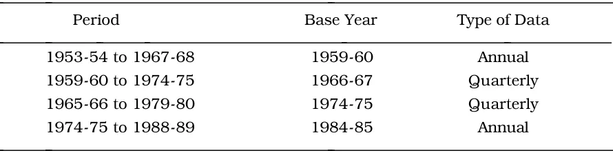
Constant-price data were based on four different constant price base years. Overlapping subintervals allowed linking of the data to a unique base year. In addition, some of the earlier constant price data were provided as quarterly data.

Current and constant-price data were not available on request for the early years of the study period. To cover the early years, data for the period 1953-54 though 1967-68 were obtained from the 1969 publications of Cat. No. 5206.0 (for current-price data) and Cat. No. 5207.0 (for constant-price data). The details regarding constant-price data are given in Table 4.2.

Table 4.2

Details of Available Constant-Price Data

Period Base Year Type of Data

1953-54 to 1967-68 1959-60 Annual

1959-60 to 1974-75 1966-67 Quarterly

1965-66 to 1979-80 1974-75 Quarterly

1974-75 to 1988-89 1984-85 Annual

The total expenditure variable in this model, M_t has been interpreted as nominal expenditure per head. Population data were obtained directly on request to Canberra from the Demographic Section of the ABS. These data were used to convert constant-price expenditure data into per capita form. There was a break in the population series at 1971 due to the introduction of an estimate of under-enumeration from the 1971 Census. This under-enumeration adjustment is included in all population figures from this time onwards. Both the original and the under-enumeration compensated figures are available for the transition year and these measures provide a fixed proportional adjustment for under-enumeration in earlier years.

The quarterly data were first aggregated to annual data and then the data were linked following the principles outlined in Adams, Chung and Powell (1988) to obtain annual real and nominal expenditure and price indices (obtained from strictly matched series) based on a constant-price base year 1984-85.

5. Results

We initially fitted AIDADS in the first differences with an error correction term (i.e., we fitted (3.2.1)); however, we present the results here in the sequence:

¥ fit in the levels without error correction18 _{(Table 5.1 and Figure 5.1)}

¥ fit in the levels with error correction (Table 5.2 and Figures 5.2 and 5.3) ¥ fit in the differences with error correction (Table 5.3 and Figures 5.4

and 5.5)

Had the results from our first estimation been fully satisfactory, it is unlikely that we would have carried out the others.

5.1 Estimation in the levels

Turning to Table 5.1, we notice that corner solutions were obtained for the α_iÊvalue for Rent, the β_i values for Alcohol and tobacco, and for Clothing and footwear, and effectively also for the γ_i values for commodities other than Food and Clothing and footwear. 19 _{Quite contrary to the findings of Theil and Clements (1987) and Adams,}

Chung and Powell (1988), these estimates show a virtually constant marginal budget share for Food over the sample.20 _{They suggest that Food's share at subsistence income}

levels wouldbe about70 per cent (viz.,p₁

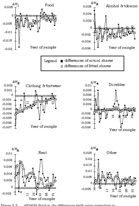
γ

_{1Ê/ (p}′γ) ≈ 0.7) with Clothing and footwear taking the remaining 30 per cent), declining to about seven percent (i.e., 100 β₁) at indefinitely high levels of affluence. Over the thirty-five year sample, the actual variation was from about 25 to about 15 per cent. The asymptotic budget share for Clothing and footwear as real expenditure grows without limit (β₃) , at zero, clearly is not sensible. Notice though that the decline over the sample from about 14 to about 6 percent of the budget is tracked relatively well (Figure 5.1).

18 I.e., equation (3.2.2) with ρ constrained to unity.

19 We have constrained the γ_is to non-negative values, even though the AIDADS system (like

LES) is interpretable outside this range. This ensures regularity for M > p′γ, albeit it at the

cost of some flexibility.

Inspection of Figure 5.1 highlights some specification problems with the model. Not unexpectedly, durables perform very poorly, with the massive changes in liquidity, in inflationary expectations, and in relative prices of the Whitlam years showing up very clearly. This is one problem which we will not be able to correct within the confines of our static model.

Overall, the most outstanding features of Table 5.1 are the high (and increasing) marginal budget share for Rent, and the pathological serial properties of the residuals (as shown in the Durbin-Watson statistics).

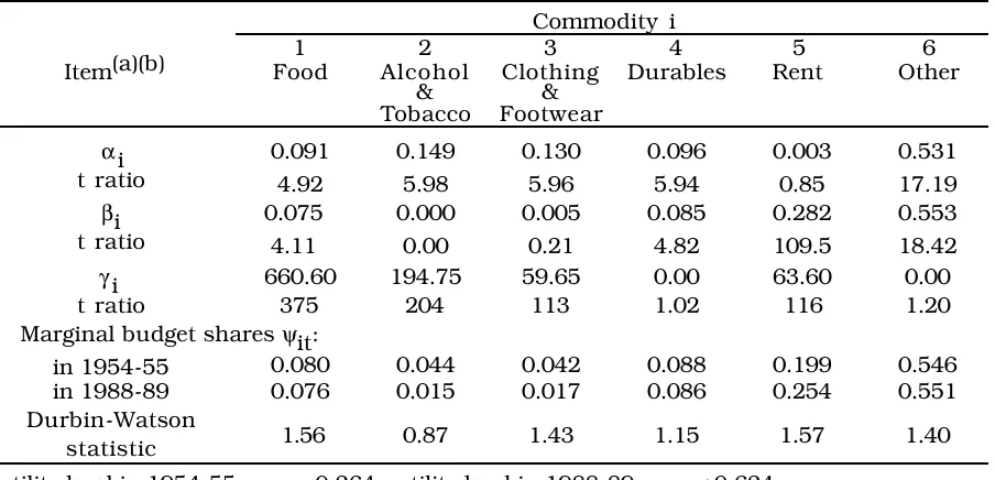
Does adding an error correction term along the lines of equation (3.2.2) help? The levels fit with error correction is documented in Table 5.2 and Figure 5.2. From the latter it will be seen that in descriptive terms the fit is excellent. The very low estimated value of ρ, namely 0.053, suggests a unit root problem. Nevertheless, the t statistic on ρ (namely, 3.3) indicates significant difference from zero. In any event, both the realized and the equilibrium values of the budget shares by construction lie within the unit interval, and hence both are I(0). The proximity of (1 Ð ρ) to unity may be caused by structural breaks in the data due to (a) the re-basing of series noted in Table 4.2 and (b) the real wage explosion of 1973-7421_.

In Table 5.2 we once again find a high marginal share for Rent which increases over the sample from 20 to 25 per cent of the budget. The final ceiling is estimated as 28.2 per cent with very high apparent precision. Relative to Table 1, several parameters change by substantial margins, but these changes are not sufficiently large to destroy the overall qualitative pattern. This surmise may be verified by comparing Figures 5.1 and 5.3, which show the equilibrium values of budget shares corresponding to the parameter values in Tables 5.1 and 5.2. The serial properties of the residuals (as shown in the Durbin-Watson statistics) are no longer severely pathological, though there is still evidence of positive serial correlation. Cross substitution elasticities are shown for the Table 5.1 parameter estimates in Table 5.4, and for the Table 5.2 estimates in Table 5.5.

5.2 Estimation in the differences

Because we anticipated positive serial correlation, and because in any event the implicit nature of the u function drove all of the analytics into differential form, it was natural for us to start by estimating the model in the first differences. The results are shown in Table 5.3 and in Figures 5.4 and 5.5.

The results in the differences yield an estimate of the error correction coefficient ρ which at O.048 is not too far away from the Table 5.1 estimate of 0.053. It is not clear that on average the serial properties of the residuals are better than those obtained in Table 5.2. The fit to the differences of the shares shown in Figure 5.4 indicates that the raw data are both noisy and spiky; the fit seems to pick up the trends, however. The larger spikes (i.e., outlying second differences) seem to be related to breaks in the basic data series. The parameter estimates, however, differ considerably from those of Tables 5.1 and 5.2.

Tables 5.1Ð5.8 and Figures 5.1Ð5.5 follow. Text resumes on page 34.

Table 5.1

Maximum Likelihood Estimates of AIDADS fitted in the Levels, Without Error Correction: Annual Australian Data, 1954-55 through 1988-89

Commodity i Item(a)(b) 1 Food 2 Alcohol & Tobacco 3 Clothing & Footwear 4 Durables 5 Rent 6 Other α_i t ratio .085 4.63 .230 27.8 .109 14.4 .156 22.1 .000 0.00 .419 31.2 β_i t ratio .077 0.44 .000 0.00 .000 0.00 .048 0.33 .294

21×103

.581 3.27 γ_i t ratio 686.28 28.9 0.53 0.68 252.87 20.4 .015 0.12 .013 0.11 .049 0.21

Marginal budget shares ψ_it:

in 1954-55 in 1988-89 .078 .077 .070 .019 .033 .009 .081 .057 .205 .269 .532 .568 Durbin-Watson

statistic 0.44 0.15 0.41 0.38 0.27 0.29

utility level in 1954-55, u1 = Ð0.348: utility level in 1988-89, uT = +0.637.

t value for u1 = -5.70.

Table 5.2

Maximum Likelihood Estimates of AIDADS fitted in the Levels, With Error Correction: Annual Australian Data, 1954-55 through 1988-89

Commodity i Item(a)(b) 1 Food 2 Alcohol & Tobacco 3 Clothing & Footwear 4 Durables 5 Rent 6 Other α_i t ratio 0.091 4.92 0.149 5.98 0.130 5.96 0.096 5.94 0.003 0.85 0.531 17.19 β_i t ratio 0.075 4.11 0.000 0.00 0.005 0.21 0.085 4.82 0.282 109.5 0.553 18.42 γ_i t ratio 660.60 375 194.75 204 59.65 113 0.00 1.02 63.60 116 0.00 1.20

Marginal budget shares ψ_it:

in 1954-55 in 1988-89 0.080 0.076 0.044 0.015 0.042 0.017 0.088 0.086 0.199 0.254 0.546 0.551 Durbin-Watson

statistic 1.56 0.87 1.43 1.15 1.57 1.40

utility level in 1954-55, u1 = Ð0.264; utility level in 1988-89, uT = +0.624.

t value for u1 = Ð7.65.

error correction coefficient Ð(1Ðρ) = Ð0.947; t value for Ð(1Ðρ) = Ð59.4.

(a) The units for the γ_is are 1984-85 Australian dollars worth of the named commodity per

head.

(b) The α_is and β_is are constrained to be non-negative and to sum to one. The γ_is are

Table 5.3

Maximum Likelihood Estimates of AIDADS fitted in the First Differences, Annual Australian Data, 1954-55 through 1988-89

Commodity i Item(a)(b) 1 Food 2 Alcohol & Tobacco 3 Clothing & Footwear 4 Durables 5 Rent 6 Other α_i t ratio .599 6.53 .310 5.24 .051 0.07 .000 0.10 .001 0.07 .038 0.93 β_i t ratio .039 0.49 .002 0.02 .048 2.70 .096 1263 .198 127 .617 21.9 γ_i t ratio 31.76 16.7 0.73 2.52 4.20 6.04 0.00 0.03 494.09 65.7 0.21 1.35

Marginal budget shares ψ_it:

in 1954-55 in 1988-89 0.085 0.047 0.027 0.006 0.049 0.048 0.088 0.095 0.182 0.196 0.569 0.609 Durbin-Watson

statistic 1.87 1.23 1.58 1.17 .65 1.50

utility level in 1955-56, u1 = 0.645: utility level in 1987-88, uT = 1.403; t value for u1 = 3.77.

error correction coefficient ρ: 0.048; t value for ρ = 4.90.

(a) The units for the γ_is are 1984-85 Australian dollars worth of the named commodity

per head.

(b) The α_is and β_is are constrained to be non-negative and to sum to one. The γ_is are

constrained to be non-negative.

Table 5.4

Estimated Substitution Elasticities for AIDADS at Beginning and End of Sample (from the Levels Estimation without Error Correction)*

i = j _Food1 _Alcohol2

& tobacco 3 Clothing & Footwear 4 Durables 5 Rent 6 Other

σ_{i i}

beginning

σ_{i i}

end

1 see last

2 cols

0.524 0.277 0.524 0.524 0.524 Ð0.82 Ð2.83

2 0.318 see last

2 cols

0.593 1.124 1.124 1.124 Ð8.88 Ð13.00

3 0.117 0.508 see last 2

cols

0.593 0.593 0.593 Ð2.72 Ð7.95

4 0.318 1.383 0.508 see last

2 cols

1.125 1.125 Ð11.01 Ð11.99

5 0.318 1.383 0.508 1.385 see last

2 cols

1.125 Ð10.00 Ð4.73

6 0.318 1.383 0.508 1.385 1.385 see last

2 cols

Ð1.46 Ð1.02

W₁

0 0.05

0.1 0.15 0.2 0.25 0.3

Food

Year of sample

W₂

0 0.02 0.04 0.06 0.08 0.1 0.12

Alcohol and Tobacco

Year of sample W₃

0 0.02 0.04 0.06 0.08 0.1 0.12 0.14

Legend

fitted share

actual share

Clothing & footwear

Year of sample

W₄

0 0.01 0.02 0.03 0.04 0.05 0.06 0.07 0.08 0.09 0.1

Durables

Year of sample W₅

0 0.02 0.04 0.06 0.08 0.1 0.12 0.14 0.16 0.18 0.2

Rent

Year of sample

W₆

0 0.05

0.1 0.15 0.2 0.25 0.3 0.35 0.4 0.45 0.5

Other

Year of sample

0 0.05

0.1 0.15

0.2 0.25

0.3

1 5 9 13 17 21 25 29 33

Food

fitted share actual share Legend

0 0.02 0.04 0.06 0.08 0.1 0.12

1 5 9 13 17 21 25 29 33

0 0.02 0.04 0.06 0.08 0.1 0.12 0.14

1 5 9 13 17 21 25 29 33

0 0.02 0.04 0.06 0.08 0.1

1 6 11 16 21 26 31

0 0.05

0.1 0.15

0.2

1 5 9 13 17 21 25 29 33

0 0.1 0.2 0.3 0.4 0.5

1 5 9 13 17 21 25 29 33

W₁

W₂

W₆

W₅

W₄

W₃

Alcohol & tobacco

Clothing & footwear

Durables

Rent

Other

Year of sample

Year of sample

Year of sample

Year of sample

Year of sample

Year of sample