Modelling and Control of KRC Systems Using
TPN and TA
H. Allaa1, H. Awad2, A. Anwar1, E. El-Hajri3
Laboratoire d’Automatique de Grenoble (INPG-CNRS-UJF), Domaine Universitaire, France1
Industrial Electronics and Control Eng., Faculty of Electronic Engineering, Minufiya Unv, Shaqra Unv., KSA2
Jubail Industrial College, KSA3
ABSTRACT: This paper models and supervises kernel railroad crossing (KRC) systems using timed Petri nets and
focuses on the control synthesis method, which consists in computing new firing conditions for the timed automaton (TA) transitions so that the forbidden locations are no longer reachable. The system to be modeled and supervised using timed Petri nets is converted to a TA and is analyzed using automata so that the functioning of the system respects given specifications. The main reason of using automata is that although the timed Petri nets supervisor controls the system, it fails to define the time units needed for the undefined time of a transition. Simulation results show the soundness of KRC modeling and supervision in the sense of ensuring the safety and maximizing utility (the gate should be opened as long as possible).
KEYWORDS: Automata, Timed automata, discrete event systems, Petri nets, Timed Petri nets, KRC systems
I.INTRODUCTION
The process synchronization and forbidden states avoidance are considered as the main problems in both normal and abnormal modes of automation systems [1]. These characteristics allow the system to be considered as Discrete Event System (DES) and allow the researchers to perform the analysis and control of such systems using Petri nets (PN) and automata. DES is a dynamic system with state evolution produced by the occurrence of physical events. For example, an event is opening or closing a gate in Kernel Railroad Crossing (KRC) systems [2-3]. DES can be found in domains such as manufacturing, robotic, traffic control, logistics, and communication systems, etc.
Important contributions in supervisory control of DES based on the Finite Automata (FA) and Petri Nets (PNs) are found in [4-8]. Petri net models are normally more compact than similar automata based models and are better suited for the representation of discrete event systems. They also have a good representational power [9]. On one hand, numerous approaches to the systematic construction of Petri net models have been proposed in [10]. On the other hand, because automata detail the process to be modelled, they are also employed to analysis and avoid forbidden states with ease.
particular event. This approach provides good solutions for the control of time discrete event systems (TDES). However, the discrete nature of time generates the exponential explosion of the number of states.
In order to solve this problem, some authors have proposed approaches based on models where the time is dense. These approaches are based on the timed automaton model. They give a solution to the TDES verification problem [13].
This paper deals with analysis and control of TDES whose behaviour is determined by the occurrence of events at moments specified by time intervals. First, it adopted the timed Petri net model (TPN) [14]. This tool inherits the modelling capacity specific to Petri nets based models. Moreover, it has the ability to represent time constraints specified by time intervals. In spite of their modelling capacity, only few properties can be determined using exclusively a TPN. The method currently used for analysing TPN properties is based on modelling its behaviour by a state class graph [14]. This tool provides an over-approximation of the TPN behaviour and it is appropriate for verification of safety properties. However, it is not adapted for control synthesis because it may represent forbidden behaviours that do not exist in the real system.
In [15], a method for building systematically the timed automaton (TA ) that models the exact behaviour of a TPN is introduced. This paper borrows this method to build a TA for KRC system. This method provides a clear graphical representation of all TPN possible forbidden behaviours and considers the forbidden states correspond to forbidden TPNs markings that are represented by forbidden TA locations.
This paper also focuses on the control synthesis of TDES modelled by TPNs that developed based on place invariants (P-invariant) [9]. The method that we propose is based on the TA with forbidden locations. For each forbidden location, the corresponding reachability path that acts on the transitions associated with controllable events is analysed. This paper also tries to define the exact time unit (t.u.) period of transitions that have undefined t.u [0, ].
The KRC is a standard benchmark in real time systems verification and operates to ensuring safety and maximizing utility (the gate should be open as long as possible) [2]. Modelling and control of KRC systems using timed Petri nets and focusing on the control synthesis method, which consists in computing new firing conditions for the timed automaton transitions so that the forbidden locations are no longer reachable, is the main contribution of this paper.
This contribution can be achieved as follows.
1- Modeling and supervising the KRC system using timed Petri nets (TPN) 2- Building the TA associated to the developed TPN
3- Analysis the TA using phaver-software
4- Control synthesis of the KRC system ensures safety and maximizes utility properties of the KRC
The paper is organized as follows. In Section II, the essential background used in this paper to TPN and timed automata is presented. In Section III, modelling and supervision of the KRC system is detailed. The main idea of building the TA associated to a TPN is described in section IV. Section V creates the TA associated with the developed TPN of the KRC system and proposes its control synthesis. Using phaver-software, simulation results are depicted in section VI. Some concluding remarks and future work are given in section 7.
II. ESSENTIAL BACKGROUND TO TPN AND AUTOMATA
Petri nets are classified based on their structural and behavioural properties [1]. Basically, a Petri net is a particular kind of bipartite directed graphs characterized by three types of objects, places, transitions, and directed arcs. The latter connects places to transitions or transitions to places. This elementary Petri net may be employed to represent various aspects of the system to be modelled. In order to study the dynamic behaviour of a system structured with a Petri net in terms of its states and state changes, each place may potentially hold with positive number of tokens. A set of definitions related to Petri nets used in this paper can be briefly discussed below [16-19].
Definition 1: A Petri net structure is a weighted bipartite graph; G
P,T,F,
, where P
p1,p2,..., pn
is atransitions and from transitions to places in the structure, and :I O
1,2,3,,...
is the weight function on the arcs.The way in which tokens are assigned to a Petri net graph defines a marking vector, M, which can be formally defined
m p m pi m pn
M 1 ,... ,..., where n, is the number of places in the Petri net. The state transition mechanism is provided by moving tokens through the Petri net and hence changing its state.
Definition 2: A transition tiT in a Petri net is said to be enabled if the number of tokens equal or exceed the weights on its output arcs, M
pi
pi,tj
,piI
tj . Since places are associated with conditions, a transition is enabled when all the conditions required for its occurrence are satisfied using a set of tokens.Definition 3: Given a Petri net with the initial marking Mo; N
G,M0
, the set of reachable states of this Petri netis called the reachability set and is signified by R
N,M0
.Definition 4: A Petri net is said to be live if it guarantees no stop operations (deadlock-freeness in general), regardless what firing sequence is chosen. Deadlock-freeness may not necessarily be completely live. A deadlocked Petri net contains at least one empty siphon. A net with an unmarked siphon is not live. For more details the reader can be directed to read [1].
In contrast to the behavioural properties defined above that depend on the initial marking vector of a Petri net, structure properties do not depend on the initial marking vector of the net. Based on the structural properties, Petri nets are classified also into many classes. These important classes are described below.
Definition 5: A state machine (finite state automata) is a Petri net in which all transitions have one input and one output place.
The timed automaton (TA) model is defined as a finite state machine extended with a set of continuous variables called clocks [14]. These variables are piece-wise continuous real-valued functions of time that precisely measure the time elapsed between events.
Definition 6: A timed automaton is 6-tuple TA= (L, L0, X,,I,T) , where: - L is the finite set of locations;
-L0 Lis the initial location; - X is the finite set of clocks;
- is a set of labels associated with the events;
- : Lm(Lm) is a mapping that associates a location invariant (Lm)with each location Lm; - T is the finite set of transitions and a transition is a 5-tuplet Tm,n(Lm,a,gm,n,Am,n,Ln)where:
m L
is the source location; ais the label associated with an event; gm,n is the firing condition, i.e. the guard; n m
A , is
the assignment;Lnis the destination location.
The clocks are synchronized and incremented while the system sojourns in a location. The dynamic of each clock x
Definition 7: Let X be the finite set of clocks. A clock valuation is a mapping
X
v: that assigns a non-negative real number to each clock.
A clock valuation defines the value of clocks at a given moment. V denotes the set of clock valuations. Let vV be a clock valuation,
t a positive rational number and Am,n an assignment. We use the notation:
• vtassigns a value v(x)tto each clock xX ; • v[Am,n] sets to zero the clocks specified by Am,n.
• v | gm,n represents the fact that the valuation v satisfies the guard gm,n of the transition Tm,n.
Definition 8: The state of a TA is defined by the pair (L, v), where L0L is a TA location and vV is a clock valuation.
A system may sojourn in a TA location Lnas long as the locations invariant (Ln)is satisfied by the value of clocks. Consequently, a location may not correspond to a state of the TA, but to a space of states. A space of clock values Q within a location Lnis called region and it is denoted by the couple (Q, Ln).
The main target of the control synthesis is to guarantee that the forbidden states or the forbidden locations, are not reachable during the evolution of the TA. Therefore, we are interested in computing: (1) the set of states reachable form a given region, called the successor of the region; and (2) the set of states from which a given region may be reached, called the predecessor of the region.
The evolution of a TA is characterized both by a continuous and a discrete dynamic. The continuous dynamic is represented by the evolution of clocks with the elapsing of time while resting in the same location. The discrete dynamic consists in transitions firing. Therefore, a region may have two kinds of successors (predecessors): continuous and discrete ones [15].
The method for computing the successors and the predecessors of a region are described in [20]. This paper uses these methods in our control synthesis approach. Although, these procedures are implemented in a software dedicated to verification of timed and hybrid systems, this paper employs phaver-software due to its power in analysing and verifying the TA model. For more details, the reader can be directed to read [15].
In the sequel this paper develops the TPN of the KRC system and its supervisor and gives the main idea of the method that used to build the TA which models the behaviour of the developed TPN.
III. MODELLING AND SUPERVISION KRC SYSTEMS USING TPN
This section develops the TPN model of the KRC and its supervisor that is synthesized based on P-invariant method [9], [21].
III.1. The KRC system description and its Petri nets
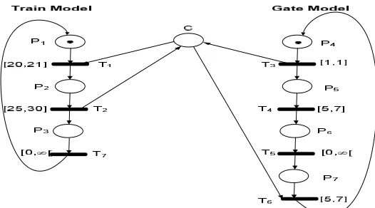
that has unknown time units "[0, ]". This is due to the reason that no expectation for beginning the departure phase of the train; its departure depends on the passenger riding. The analysis should be performed to get the exact period time unit required to activate the transition T5 every departure phase. This means that this transition is continuously evaluated as detailed in the subsequent sections. The system comprises two tasks, train task and gate task. We consider that the controllable events are the beginning of each task. However, the accomplishing of the tasks is uncontrollable. Therefore, our goal is to control the beginning of the tasks in order to obtain safe arrival and departure of the train. Also, the synthesized control scheme should avoid the forbidden state (P2, P4). This means that the train in the R-Y zone and the gate still opened.
Fig. 1. A kernel railroad crossing system
Fig. 2. The simplified Petri net model of Fig. 1
Table 1
The recipe of the Time Petri net (Fig.2)
Place Associated action Tr. Associated event
P1 The train arrived at the first point of the R-Y zoon
T1 Inter the R-Y zoon
P2 The train in the R-Y zoon
T2 Exit the R-Y zoon
P3 The train exit the R-Y zoon
T3 Go-down
P4 Gate is completely opened
P5 Gate is closing T5 Go-up P6 Gate is completely
closed
T6 Stop go-up
P7 Gate is opening
Fig. 3. The time Petri net of the KRC (Fig. 1)
III.2. Analysis the PN of the KRC system
Using Petri net tool software ver. 2.1, the system incidence matrix is:
1 1 0 0 0 0 0 1 1 0 0 0 0 0 1 1 0 0 1 0 0 1 0 0 0 0 0 0 1 0 0 0 0 0 1 1 0 0 0 0 0 1 PW
III.3. Supervisory Control Synthesis for the KRC system
This subsubsection develops the supervisory control scheme that aims to restrict the reachable markings of a plant,
m
psuch that:
B
Lmp (1)
where
m
p is the marking vector of the plant,n nc
L , Bnc, nc c
M and
n
c is the number of constraints to beenforced on the plant model. The system to be controlled is modelled by a Petri net with
n
places andm
transitions. For more details about Petri nets, the readers can be directed to read [5], [16], [21]. The incidence matrix of the plant ism n p
D
. It is possible that the process net violates certain constraints posed on its behaviour and it needs some of
supervision. So, the inequality defined in (1) can be transformed into the equality defined in (2) by introducing a nonnegative slack variable
M
c into this equation. Then (1) becomes:B M
Lmp c (2)
The slack variable
M
c in this case contains new places that hold the extra tokens required to meet the equality. The slack variable that enforces the equality defined in (2) is a part of a separate net called the supervisor (controller). If the initial marking does not violate the given set of constraints defined in (1), these constraints can be enforced by the supervisor with the incidence matrix [4].P
C LD
D (3)
The initial marking of the proposed supervisor is computed by:
0
0 p
C B Lm
M (4)
where
m
p0 is then
1
initial plant marking vector of non-negative integers. The supervisor is a Petri net with incidence matrix Dc made up of the process net's transitions and a separate set of supervisor places. The supervised net is also called the controlled system or the closed loop system and is defined as: C p D D
D and C p M m
m (5)
Uncontrollable transitions cannot be prevented from firing by the supervisor. They can cause problems for the PN based supervisors due to limitations in their modeling power. For an invariant-based Petri net supervisor to be realizable on a plant with uncontrollable transitions, the constraints enforced by the supervisor must be admissible. Inadmissible constraints cannot be directly enforced on a plant due to the uncontrollability of certain plant transitions. Procedures are given for identifying all admissible linear constraints for a plant with uncontrollable transitions, and methods for transforming inadmissible constraints into admissible.
Let Duc be a matrix representing the columns in the plant incidence matrix that corresponds to uncontrollable transitions. The matrix LDuc must contain non-positive elements when constructing the supervisor. Thus for the constraints to be admissible, it must satisfy:
0
uc
LD (6)
If this is not the case, matrix L and vector B must be transformed so that (6) is to be satisfied, while the supervisor designed to enforce the new set of constraints that will also maintain the original set of constraints. This can be
achieved by performing row operations on Duc and LDuc. Matrices R1 and R2 are used to transform the inadmissible
constraints Lmp B into the admissible constraints [4]:
'
'm B
L p (7)
where L R R
L' 1 2 and B'R2(B) (8)
Such that ncn R
1
0
1
Rmp and R2Zncnc is a positive definite diagonal matrix, and I is
n
cvector.To illustrate the idea of the proposed supervisory control scheme, let us consider the constraint defined below. 1
4 2m
The constraints vector is L
0 1 0 1 0 0 0
, the controller incidence matrix is
1 1 1 0 0 1
p
c LW
W , the initial marking of the controller is mc0 BLm0 0, and B1.
The developed supervised time Petri net of the KRC system is depicted in Fig. 4. There are 10 reachable states starting from the initial marking vector M0 to the final vector M10 and the supervisor eliminates the forbidden state vector M = [0,1,0,1,0,0,0].
Eliminating the forbidden state is the first objective of this paper, however, determining the time units required for the transition T5 is also its second objective. So, the timed Petri net shown in Fig. 4 is converted to a timed automaton for analysing purposes. This analysis should eliminate the forbidden state (location) and determine the time unit of the transition T5. This matter is detailed in section 5.
Fig. 4. The supervised timed Petri net of the KRC (Fig. 1)
IV. TPN AND TIMED AUTOMATA
This section describes the relation between TPN and TA. It also designs a TA for the KRC system and its control synthesis.
IV.1. TPN and TA relationship
In a TPN, the occurrence of an event is subject to time constraints similar to that of TA [22]. Thus, a transition may be fired if it is enabled by a marking vector and if some time constraints are satisfied [14], [23]. The marking vector remains unchanged between two consecutive transition firing. Thus, each marking vector of the TPN can be modelled by a TA location, while the firing of a TPN transition can be modelled by a TA transition. The time information memorized by a time Petri net can also be represented by elements of a timed automaton as follows. First, the time elapsed since a transition enabling moment is measured by a clock. Second, the time interval of a TPN transition is modelled by the guard of the corresponding TA transition. Third, the initialization of the clocks associated to the newly enabled transitions is modelled by the assignment of the corresponding TA transition. Thus, the behaviour of a TPN be can be modelled by a TA.
the solution is to dynamically allocate with each transition a number of clocks equal to the number of simultaneous enabling.
IV.2. Elements of a TA
The elements of the TA which models the behaviour of a TPN are described as follows:
IV.2.1. Locations
Each TPN marking vector Miis modelled by a unique TA locationLi.
IV.2.2. Clocks
A clock xj is associated with each TPN transitionTj. It serves to count the time elapsed since the last enabling moment of the transition Tj and determines if the firing condition of this transition is satisfied or not.
IV.2.3. Transitions
Firing a TPN transition is modelled by a TA transition. The guard of the TA models the firing interval of the TPN transition while its assignment initializes the clocks associated with the newly enabled TPN transitions.
4.2.4. Constructing the TA associated with a TPN
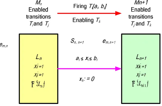
The initial TPN marking vector is modelled by the TA initial location. The TA is structured by analysing the evolution of the TPN from its initial marking vector. Fig. 5 depicts the principle of the building method.
1
Ln
Ln
Fig. 5. The principle of the TA structuring
IV.2.5. Computing a location invariant
The location invariant (Ln) is stemmed from the time intervals of the transitions Ti and Tj, and is enabled by the marking vector Mn.
To clarify this point, if the firing interval of Ti is [ai, bi], then Ti cannot be continuously enabled more than bi t.u.
system may sojourn in Lnas long asxj bj. The invariant of Ln is (Ln)0xi bi and0xj bj. Thus, the evolution of the time is never stopped and the TA is non blocked as mentioned in section 3.
IV.2.6. Calculating the space of clocks in a location
When a locationLnis reached by firing a transitionTm,n, there are a set of possible values for the clocks. These values
define the space of clock values denoted byEm,n. The space of clocks within a locationLn, denoted Suc(Em,n) is the continuous successor of the space of clocks at the access of Ln.
Property 1: The space of clocks in a location Lnrepresents the set of all possible evolution trajectories while the system sojourns in Ln [15].
V. CREATING A TA FOR THE TPN
This section develops the TA associated with the developed TPN of the KRC system. It also creates a timed automaton transition and defines the space of clocks at the entrance of a location.
V.1. A timed automaton transition and the space of clocks
A timed automaton transition can be created by firing the ith transition Ti using the marking vector Mn to lead the marking vectorMn1. This creates a new location Ln1 which models the marking vector Mn1. Firing the TPN transition Ti is modeled by a TA transition Tn,n1 which links the locations LnandLn1. If the firing interval of the transition the transition Ti is [ai,bi], the guard of Tn,n1 is gn,n1[ai xi bi]. The evolution of the TPN marking vector owing to the firing of the transition Ti has enabled Tk. Accordingly, the assignment of Tn,n1should initialize the clock xk associated with Tk:An,n1[xk:0], where An,n1 is the assignment
The space En,n1of clocks at the entrance of the locationLn1 by firing the transition Tn,n1is the discrete successor of the space Sn,n1:En,n1Sucn,n1(Sn,n1). The set of the active clocks values which verify the guard
1 ,n
n
g
of the TA
transition Tn,n1, which links the locations Lnand Ln1, denoted by Sn,n1is g n n n m n
n SucE
S , 1 ( , ) , 1where Suc(Em,n) is the space of clocks in the locationLn. The method employed for computing the continuous and discrete successors of a space of clocks values can be found in our previous work [15].
V.2. The timed automaton of the KRC system
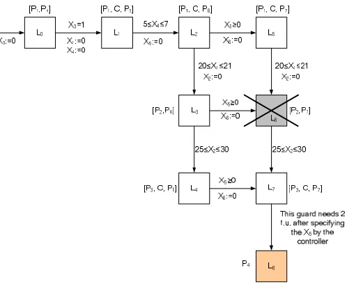
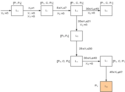
This subsection constructs the TA associated with the developed TPN. Fig. 6 models the exact behaviour of the TPN developed in this section 3 and depicted in Fig. 4. Our goal is to avoid the forbidden state (location 6; L6) and to define
the proper guard g3,6 to define the right period of the transition T5 depicted in Fig. 4.
A clock xi is associated with each TPN transition Ti. The initial TA location L0corresponds to the state where the train arrived at the first point of the R-Y zoon and the gate of the KRC system is completely opened. Let us suppose that the train in the R-Y zoon, P2, and the gate starts its opening task by firing the transition T5, the system reaches the
forbidden location L6. These forbidden locations must be avoided. Avoiding these states solves two problems addressed by this paper, the forbidden states and infinity problem that is defined as "T5 [0,]". It also achieves the safety and utility properties of the system. Therefore, the clocks of the transitions that link L3 and L6 should be determined and consequently the time units of the transition T5 can be determined. These problems will be solved in
Property 2: The TDES forbidden behaviors are modeled by forbidden locations.
Property 3: The guard gm,n of each transition Tm,n is described by an expression gm,n [aixi bi], where xi is a clock and ai, bi are rational numbers.
Property 4: The TA constructed by this method is non blocking.
Fig. 6. The TA associated with the developed TPN (Fig. 4)
V.3. The control synthesis of the KRC system
In time discrete event systems (TDES), events are classed according to the possibility to control their occurrence dates into three kinds, controllable, uncontrollable and forcible [12], [15]. In this paper, the first two types are more adapted to TDES control. An event is said to be controllable if it is possible to fix its occurrence instant within a given time interval. In contrast to the controllable events, an event is considered to be uncontrollable if it is not possible to act on its arriving moment (sensors). The time interval associated with an uncontrollable event may be considered as an uncertainty on its arriving moment. The aim of the control synthesis is to compute new time constraints on the occurrence of controllable events so that the functioning of the KRC system respects the specifications. Synthesizing the controller for the KRC system is detailed below.
The TDES control synthesis method proposed is based on the timed automaton model respecting the properties presented in section 4. Each timed automaton transition models the occurrence of an event and its guard models the time constraint imposed on the occurrence of the associated event. The main idea of synthesizing the proposed controller in this paper is to modifying the time constraint associated with a controllable event. By this modification this event occurrence at certain time instants can be forced such that the functioning of the system follows the desired specifications. Also, the time units needed for the unknown time units transitions e.g. T5 and its clock x5 in our application can be determined.
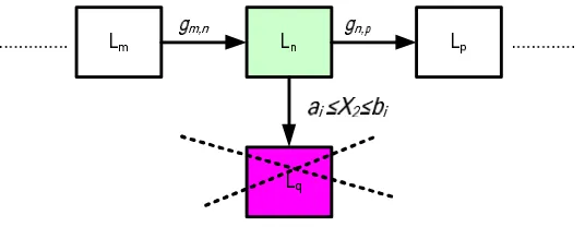
The control synthesis method proposed in this paper comprises two steps, analysing one by one each forbidden location, and computing new guards for the controllable transitions so that the forbidden location is not reachable. It is executed in two phases, forward treatments and backward treatment. The principle of this method using the part of a timed automaton depicted in Fig. 7. In this figure, the forbidden location Lq can be reached from Lnby firing the transition, Tn,q. The main objective of the control synthesis method is to avoid the forbidden locations in general e.g.
q
L in this situation. Therefore, the system must leave the location Lnby firing another output transition leading to the not forbidden locationLp. So, this firing condition should be forced before the guard of the transition Tn,q becomes
enabled by the value of clocks. Another important pint is that if the transition Tn,q to the forbidden location is
uncontrollable, its guard cannot be modified and we must compute a new initial condition of the continuous dynamic of clocks in the location.
Fig. 7. Part of a timed automaton with a forbidden location
As mentioned above, the control synthesis is executed in two phases, forward treatments and backward treatment. The former concerns only the locationLn. This subsection can be summarizes the scheme as follows.
- The forward treatment phase
If a transition Tn,p is controllable, compute a new guard
d p n
g , for the transition Tn,pin order to force the firing of this
transition before the guard of the transition Tn,q becomes satisfied by the clocks and update the location invariant
) (Ln
according to the new guard computed for the transition Tn,p.
1- Compute the space of desired clock values, d n
D in the location Ln. This step restrains the space of clocks values in the location Ln so that the guard gn,qof Tn,qis never verified during the sojourn of the system in this
location.
2- Compute the space d n
E of the desired clock values, d n
D at the entrance of the locationLn. This new space symbol, d
n
E , is due to the fact that the space of desired clock values, d n
D within a location is characterized by the continuous dynamic of clocks and the initial condition for this dynamic. The former is fixed. The only way to modify the space of clocks values in location Lnis to act on the initial condition, i.e. the space Enof clock values at the entrance of Ln. The space of desired clock values has three situations:
(a) If d n n E
E then the space clock values within the location Lndoes not allow the KRC system to reach the forbidden location Lq. Thus, the control synthesis problem for Lqis solved.
(b) If d n
E then the evolution from Lnto the forbidden location Lqcannot be avoided and the former becomes a forbidden location.
(c) If the conditions (a) and (b) cannot be satisfied i.e. d n n E
E and d n
- The backward treatment phase
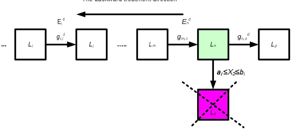
The backward treatment consists in going back in the automaton structure and compute new guards for controllable transitions such that all possible clock values at the entrance of the location Lnbelong to d
n
E . The main idea of the backward treatment is shown in Fig. 8. It can be summarized as follows.
Fig. 8. Principle of the control synthesis in its backward phase
This phase goes back through a set of locations as shown in Fig. 8. Suppose that this backward phase reaches the location Lj and computes the desired space clock values d
n
E . 1- If a transition Ti,j is controllable, compute a new guard
d j i
g, and update the location invariant (Ln)
according to the new guard computed for the transition Ti,j. 2- Compute the space of desired clock values, d
i
D in the location Li. 3- Compute the space d
i
E of the desired clock values, d i
D at the entrance of the locationLi. The space of desired clock values has three situations:
(a) If d i i E
E then the space clock values within the location Lidoes not allow the KRC system to reach the forbidden location Lq. Thus, the control synthesis problem for Lqis solved.
(b) If d i
E then the locationLi becomes a forbidden location. (c) If the conditions (a) and (b) cannot be satisfied i.e. d i
i E
E and d i
E and if Li not equals the initial location, L0 then go one transition backward in the automaton structure and return to the step #1, otherwise the control synthesis cannot avoid the forbidden stateLq.
VI. SIMULATION RESULTS AND DISCUSSIONS
This section simulates the proposed control synthesis on the KCR system using phaver software. The scheme changes the guards of the forbidden states if its transition is controllable or modifies the initial conditions otherwise. Using phaver software, the space of clocks values before starting the control synthesis procedure is shown in Fig. 9. This figure shows that the location L6 is forbidden state and must be avoidable. To avoid this forbidden state, two guards,
6 , 3
g and g2,5 must be changed if the transition T5 is controllable, otherwise the backward treatment phase is applied to reinitialize the KRC system. Let us consider the transition T5 is controllable; the forward treatment phase detailed in section 5 is employed. Fortunately, changing the guard g3,6 is enough in our application due to its similarity with g2,5
Fig. 9. Space of clock values in L6before control synthesis.
The philosophy of the control synthesis proposed in this paper is that determining the clock space of the unknown transition time unit e.g. T5 shown in Fig. 4 and consequently avoiding the forbidden locations. Suppose that a transition
6 , 3
T is controllable, compute a new guard d
g3,6 to satisfy the property 3 in order to force the firing of the transition T3,6
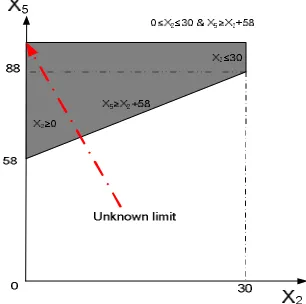
after the guard of the transition T3,4 becomes satisfied by the clocks. Starting with the controlled system behaviour shown in Fig. 10, the space of clocks values in L6for the new guard g3,6 is X2 12X5X2 16. It is to be noticed that there still remains some clocks values can be modified to lead the optimal clocks.
Fig. 10. Space of clocks values in L6for the new guard g3,6
Running the control synthesis with new conditions, leads to the space of clocks values in L6 for the new guard g3,6 is 10
2 5 2 X X
X as depicted in Fig. 11. In This figure, at X2=30, the guard g3,6 becomes g3,6
30X5 40
.Consequently, the guard g7,8 can be estimated based on its t.u. needed; 2 t.u. Accordingly, it becomes
40 5 42
8 ,
7 X
Fig. 11. Space of clocks values in L6for another new guard g3,6
Updating the location invariant (L6) according to the new guard computed for the transition T4,6, is as follows. The maximum and minimum limits of the location invariant (L6) can be updated using (10) and (11) respectively.
( 10)
) ( )
( 6 6 5 5
L L X X (10)
( )
) ( )
(L6 L6 X5X2
(11)
Compute the space d
E6 of the desired clock values at the entrance of the locationL6 as follows. 6
6
6 D E
Ed
where E6
20X121
X2X5 X2 10
, and
6
20 1 21
2 5 2 10
6 SUCE X X X X
D
Using phaver-software, leads to the result that the desired space is E6 E6&
d . Thus, the control synthesis problem
for L6 is solved with its new guard and there is no need to the backward phase. Furthermore, by applying the control synthesis method for this forbidden location, the TA for the control of the KRC system is obtained and shown in Fig. 12. Compared with Fig. 6, the forbidden location L6 is eliminated. Also, the number of locations is decreased that helps in searching purposes over the TA of the system.
This paper discussed TDES modelling and control using Petri nets and automata. P-invariant based supervisor was designed to control the Petri net model of the KRC system. Although this method controls the system, it fails to define the time units needed for the undefined transition, "T5=[0, ]". A timed automaton model that represents the
supervised Petri net model of the system is developed to overcome this problem. Phaver- software was employed for analysing the developed TA model and defining the guards of each transition. The proposed
scheme ensures safety and maximizes the utility property.
The issues initiated in this paper are discussed and solved using a simplified Petri net model of the KRC system. The proposed supervisor and TA scheme of the KRC system is valid for more complicated cases as depicted in Fig. 13. In this case, the authors supposed that the process is reversible. This assumption increases the forbidden locations by one and constructs a more complex TA model. Based on the methods proposed in this paper, the TA associated with the TPN built in Fig. 13 is depicted in Fig. 14. To avoid the repetition and due to the lack of space, the researchers who are interest can perform the same analysis made in this paper to the TA developed and depicted in Fig. 13 using the control synthesis proposed in this paper. Therefore, using phaver-software, the space of clocks values of locations should be defined to avoid the forbidden state L11 and L12 respectively. To avoid these forbidden states, all guards must be also computed and updated if the transitions T5 and T7 is controllable, otherwise the backward treatment phase is applied to reinitialize the KRC system.
Fig. 13 The reversible supervised time Petri net of the KRC
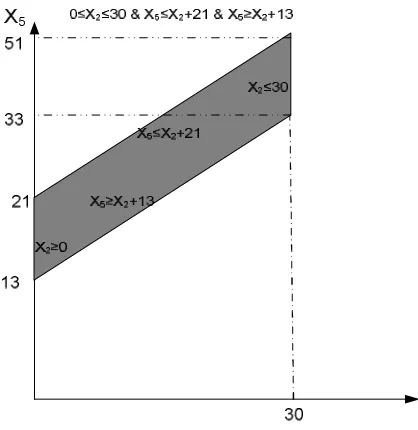
Figs. 15 shows the final space of clock values of locations L5 as an example. This guard should be updated to prevent
the firing transition T8,12. In this case, the guard g5,8
X213X5X221
at 0x2 30, becomes
13 5 51
6 ,
3 X
g . Compute the space d
E8 of the desired clock values at the entrance of the locationL8 as follows. 8
8
8 D E
Ed , where E8
20X121
X213X5 X221
and
8
20 1 21
2 13 5 2 21
8SUC E X X X X
Fig. 14 The TA associated with the developed TPN (Fig. 13)
Fig. 15. Space of clocks values in L5 at 0x230
Fig. 16 The final developed TA associated with the TPN (Fig. 13)
VII.CONCLUSIONS
This paper modelled and supervised the kernel railroad crossing (KRC) system using timed Petri nets. The developed Petri net model is analysed using its timed automata so that the functioning of the system respects a given specification. This paper also proposed the control synthesis method, which consists in computing new firing conditions for the timed automaton transitions so that the forbidden states are no longer reachable. The proposed control synthesis comprises two phases, forward and backward. Simulation results using phaver-software shows the effectiveness of the proposed controller for TDES for ensuring the safety conditions of the system and for maximizing the utility property. Although the KCR is employed for testing the proposed scheme, it is valid for more complex systems. Extending the proposed scheme to more complex problems is our future work. Furthermore, the malfunction of sensors, actuators, and erroneous actions of human operators can have some disastrous consequences in high risk systems [24-27]. These faults can lead to undesirable actions. Our future work also is to design and implement fault detection and isolation schemes for the KRC systems.
REFERENCES
[1] T. Murata, "Petri Nets: Properties, Analysis and Applications", Proceedings of IEEE, Vol. 77, pp.541-580, 1989
[2] J. S. Fitzgerald, A. E. Haxthausen, H. Yenigun, Theoretical Aspects of Computing, Berlin Heidelberg, Germeny, ISBN: 978-3-540-85761-7, 2008.
[3] C. A. Furia, D. Mandrioli, A. Morzenti, M. Rossi, Modelling Time in Computing. Springer-Verlag Berlin Heidelbrg, Germeny, ISBN: 978-3-642-32332-7, 2012.
[4] M. M. Gomaa, H. A. Awad, A. R. Anwar, "Design and Implementation of Supervisory Control Schemes in Industrial Automation Systems",
Proceedings of IEEEInternational Conference on Computer Engineering and Systems, ICCEC'08, pp. 398-404, 25-27, Cairo, Egypt, 2008. [DOI:
10.1109/ICCES.2008.4773035]
[5] P. Linz., "An Introduction to Formal Languages and Automata", Jones and Barteltt Publications, Sundbury, Massachusetts, 2001.
[6] I. Demongodin, N. T. Koussoulas, “Differential Petri Net models for industrial automation and supervisory control,” IEEE Transaction on
Systems, Man, And Cybernetics, part c: Application and Reviews, vol.36, no.4, 2006. [DOI: 10.1109/TSMCC.2005.848154]
[7] L. Ghomri, and H. Alla, "Modeling and Analysis using Hybrid Petri Nets" Nonlinear Analysis: Hybrid Systems, vol. 1, Issue 2, pp. 141-153, 2007.
[8] H. A. Awad, " Developing a Parallel Model for Oil Producing Processes " Asian Transactions on Engineering, Pakistan, vol. 01, Issue 05, ISSN 2221-4267, pp. 1-16, November, 2011.
[9] M.V. Iordache and P.J. Antsaklis. Supervision Based on Place Invariants: A Survey, Technical Report of the ISIS Group at the University of Notre Dame ISIS-2004-003, 2004.
[10] M. D. Jeng, and F. DiCesare, “A Review of Synthesis Techniques for Petri Nets with Applications to Automated Manufacturing Systems”, IEEE
[11] D. Kezic, I. Vujovic, and I. Kuzmanic, “Maximally Permissive Supervisor of Marine Canal Traffic System”, Proceedings of the IEEE, Conference for Intelligent Transportation Systems and Control, ITSC'06, Toronto, Canada, pp.1424-1429, Sept. 2006. [DOI:
10.1109/ITSC.2006.1707423]
[12] B. Brandin, and W.M. Wonham, "Supervisory Control of Timed Discrete Event Systems", IEEE Transactions of Automatic Control, vol. 39, pp. 329–341, 1994.
[13] K. Altisen, G. Goesler, A. Puneli, J. Sifakis, S. Tripakis, and S. Yovine, "A Framework for Scheduler Synthesis", Proceedings of the 1999 IEEE,
Real-Time Systems Symposium, Phoenix, AZ, USA, 1999. [DOI: 10.1109/REAL.1999.818838]
[14] B. Berthomieu, and M. Diaz, "Modeling and Verification of Time Dependent Systems using Time Petri Nets", IEEE Transactions on Software
Engineering, vol. 17, pp. 259–273, 1991.
[15] A.T. Sava and H. Alla, "A Control Synthesis Approach for Time Discrete Event Systems", MathematicsandComputersinSimulation, vol., 70, pp. 250–265, 2006. [DOI: 10.1016/j.matcom.2005.11.001]
[16] R. David and H. Alla, Discrete, Continuous, and Hybrid Petri Nets, ISBN: 3-540-22480-7, Springer-Verlag, Berlin Heidelberg, 2005. [17] R. David and H. Alla, "Petri Nets for Modeling of Dynamic Systems :A survey", Automatica, ISSN:0005-1098, vol. 30, pp. 175-202, 1994. [ DOI bookmark: 10.1016/0005-1098(94)90024-8].
[18] B. Hrúz and M.C. Zhou, Advanced Textbooks in Control and Signal Processing: Modeling and control of discrete-event dynamic systems,
ISBN-13: 9781846288722, Springer-Verlag London Limited, 2007.
[19] C. H. Chen and J. H. Dai, "Design High-Level Synthesis of Hybrid Controller", Proceedings of the IEEE International Conference on
Networking, Sensing, and Control, Taipei, Taiwan, vol. 1, pp. 433-438. [DOI: 10.1109/ICNSC.2004.1297477], 2004.
[20] S. Yovine, "Model Checking Timed Automata", In: G. Rosenberg, F. Vaandrager (Eds.), Embedded Systems, LNCS, p. 1494, 1998.
[21] J. O. Moody and P. J. Antsaklis, Supervisory Control of Discrete Event Systems Using Petri Nets, Kluwer Academic Pub., ISBN-13:
978-0792381990, 1998.
[22] R. Alur, and D.L. Dill, "A theory of Timed Automata", Theoretical and Computer Sciences, vol. 126,183–235, 1994.
[23] P. Merlin, and D. J. Faber, "Recoverability of Communication Protocols: Implications of a theoretical study", IEEE Transactions on
Communications, vol. COM-24, 1976. [DOI: 10.1109/TCOM.1976.1093424]
[24] J. Arámburo-Lizárraga, A. Ramírez-Treviño, E. López-Mellado, and E. Ruiz-Beltrán, Fault Diagnosis in Discrete event Systems using
Interpreted Petri Nets, Advances in Robotics, Automation and Control, Book edited by: J. Arámburo and A. Ramírez-Treviño, ISBN
78-953-7619-16-9, pp. 69-84, I-Tech, Vienna, Austria, 2008.
[25] L. Elshenawy, and H. A. Awad, "Recursive Fault Detection and Isolation Approaches of Time-Varying Processes ", Industrial & Engineering
Chemistry Research, vol. 51, Issue 29, pp. 9812-9824, 2012. DOI: 10.1021/ie300072q.
[26] F. Basile, P. Chiacchio, and G. De Tommasi, “An Efficient Approach for Online Diagnosis of Discrete Event Systems”, IEEE Transaction on
Automatic Control, vol. 54, pp. 748-759, 2009. [DOI: 10.1109/TAC.2009.2014932]
[27] E. AlHajri; H. A. Awad, “An Efficient Multiple Fault Detection and Isolation Scheme for Discrete Event System”, International Journal of
Automation and Power Engineering (IJAPE), Vol. 3 Issue 1, 2014. [DOI: 10.14355/ijape.2014.0301.09]
BIOGRAPHY
Prof. Hamdy Ali Ahmed Awad received the B.Sc. degree in Industrial Electronics, and the M.Sc. degree in Adaptive Control Systems from Faculty of Electronic Engineering, Minuf, Minufiya University, Egypt in 1988 and 1994 respectively.
Prof. Awad received the Ph.D. degree in Artificial Intelligent Systems in 2001 from School of Engineering, Cardiff University, Cardiff, Wales, England.
Prof. Awad has got Associative Prof. degree in Computer Sciences and Control Systems in 2007, Egypt.
Prof. Awad has got Prof. also degree in Computer Sciences and Control Systems in 2014, Egypt. Since August 2007, Prof. Awad has been with the Faculty of Electronic Engineering, Minufiya University, Egypt and King Saud University, KSA. Since 2011, He works in Shaqra University, KSA.