Data Pruning of Tomographic Data for the Calibration of Strain Localization Models

Article

Data pruning of tomographic data for the calibration of

strain localization models

William Hilth1*, David Ryckelynck1and Claire Menet2

1 2

3 4 5 6

7 8

1 _{MinesParisTech,PSLResearchUniversity,MAT-CentredesMatériaux,CNRSUMR7633,BP8791003Evry,France}

2 _{UniversityofLyon,INSAdeLyon,UMRCNRS5510,Villeurbanne,France}

* Correspondence:[email protected]

Abstract: ThedevelopmentandgeneralizationofDigital VolumeCorrelation(DVC)onX-raycomputed tomographydatahighlighttheissueoflongtermstorage.Thepresentpaperproposesanewmodel-freemethod forpruningtheDVCdata.Thesizeoftheremainingsampleddatacanbeuser-defined,dependingontheneeds concerningstoragespace. Thedatapruningprocedureisdeeplylinkedtohyper-reductiontechniques. The DVCdataofaresin-bondedsandtestedinuniaxialcompressionisusedasanillustratingexample.

Therelevanceofthepruneddataistestedafterwardsformodelcalibration. AnewFiniteElementModel Updating(FEMU)techniquecoupledwithanhybridhyper-reductionmethodisusedtosuccessfullycalibratea constitutivemodeloftheresinbondedsandwiththepruneddataonly.

Keywords:Archive;ModelReduction;3DReconstruction;InverseProblemPlasticity;DataScience 9

1. Introduction 10

With the development and the generalization of digital image correlation (DIC) or digital volume 11

correlation (DVC) techniques on Computed Tomography (CT) data, the volume of data acquired has drastically 12

increased. This raises new challenges, such as data storage, data mining or the development of relevant 13

experiments-simulations dialog methods such as model validation and model calibration. 14

In experimental mechanics, the access to full 3D fields like displacement or strain fields is far richer than 1D 15

load-displacement curves. These data can drive finite element simulations for model calibration. Although 16

extremely convincing, the increasing resolution of the full-field measurement tools, such as X-ray Computed 17

Tomography, leads to an explosion of the volume of data to store. The long term storage of CT data sets is 18

nowadays an issue (see van Ooijenet al.[1]). 19

This paper proposes a numerical method for pruning 3D data set related to DVC when it becomes necessary 20

to free up storage capacity. It aims to preserve the ability to identify constitutive equations reflecting strain 21

localization. It is a mechanical based approach to prune DVC data. Original experimental data are preserved 22

solely in a reduced experimental domain (RED). 23

Compression of data is known to be a convenient approach to restore storage capacity. For instance, MP3 24

files are a fairly common way to reduce the size of audio files for a daily use (see Pan [2]). However, a non 25

negligible loss of information is needed, but controlled. The MP3 compression roughly consists in filtering 26

certain components of the non-reduced audio file that are actually non-audible for most people. In other words, 27

the MP3 algorithm was made to prune the audio data that are not absolutely necessary. Usually the compression 28

rate is around 12. In the same philosophy, there can be a way to massively compress the experimental data 29

taken from experiments with a controlled loss of information based on an algorithm that detects the pertinent 30

information. This has been proposed in Cioaca and Sandu [3] by using a sensitivity analysis with respect to 31

variations of calibration parameters. These parameters are the coefficients of a given model that should reflect 32

the experimental observations. The result is that the pruned data are dedicated to a given model. In this paper, 33

a model-free approach is proposed. It aims to make possible various calibrations with different models after 34

data pruning. Here, the relevant information are local but situated in regions submitted to strain localization. 35

The data submitted to the pruning procedure are the outputs of a Digital Volume Correlation that reconstructs 36

the displacement fieldu(x,t)for observations at time instants(tj)j=1,...Nt, over a spatial domainΩ, wherex 37

is a position vector. The geometry of the experimental sample is approximated by a mesh and the determined 38

displacement is decomposed on finite element (FE) shape functions [4]. 39

The proposed method can be linked to data pruning or data cleaning methods described in the literature for 40

machine learning [5]. The aim of these procedures are not to reduce data storage but to improve the data quality 41

by accurate outliers detection for instance [6]. In Honget al.[7], a data pruning method is employed to filter the 42

noise in the data set. 43

Using the FE approximation of the experimental fields paves the way to further simulations. In the calibration 44

procedure, the full-field measurements are used as inputs of an inverse problem that aims to determine a given set 45

of parametersµ={µ1, . . . ,µm}. These parameters are the coefficients of given constitutive equations. Their 46

values are unknown or not known precisely. The most straightforward method is called Finite Element Model 47

Updating (FEMU) (see Kavanagh and Clough [8], Kavanagh [9]). It is a rather common way to optimize a 48

set of parameters taking into account the experimental data and balance equations in mechanics. It consists in 49

computing the discrepancy between the FE approximation of the experimental fields and the FE simulations. 50

Thus, an optimization loop is done onµwhere the FE method is used as a tool for assessing the relevance of the 51

parameter set. The objective function, or cost function, of the optimization can focus on the difference between 52

the computed and experimental displacement fields (FEMU-U), forces (FEMU-F, or force balance method), or 53

the strain fields (FEMU-ε) or a mix between all these sub-methods. A review of FEMU applications can be found 54

in Iennyet al.[10]. The method is particularly suitable for: 55

• Non-isotropic materials (e.g.: orthotropic materials in Lecompteet al.[11] or Molimardet al.[12] or 56

anisotropic materials such as the human skin [13]) ; 57

• Heterogeneous materials such as composites [14]; 58

• Heterogeneous tests like open-hole tests (e.g.: Lecompteet al.[11], Molimardet al.[12]) or CT-samples 59

[15]; 60

• Special cases of local phenomena like strain localization or necking (e.g.: Forestieret al.[16], Gitonet al. 61

[17]) or the illustrating case of the present paper; 62

• Multi-materials configurations (e.g.: solder joints studied in Cugnoniet al.[18] or heterogeneous material 63

identification done in Latourteet al.[19]); 64

• Determination of the boundary conditions [20]. 65

One of the recent developments concerning FEMU is to couple this method with reduced order models 66

(ROMs) to cut down the computation time in the parameters optimization loop. An example of such recent 67

developments can be found in Neggerset al.[21] where a method called FEMU-b is highlighted, or in Cugnoni 68

et al. [22]. The FEMU-b consists in determining an intermediate space of predominant empirical modes 69

associated to a reduction procedure, like the Proper Orthogonal Decomposition (see Aubryet al.[23]) or the 70

PGD [24]. The discrepancy is computed between the experimental and simulated reduced variables, where the 71

reduced variables are solutions of reduced equations. 72

In Ryckelynck [25], it has been shown that ROMs can be supplemented by a reduced integration domain, by 73

following the hyper-reduction method. This leads the way for for data pruning methods that preserve calibration 74

capabilities. Here, the dimensionality reduction of experimental data enables the restriction of experimental data 75

to a reduced experimental domain (RED). This RED is a subdomain of the specimen where the experimental 76

data are sampled. It is not necessarily a connected domain. The calibration capabilities of the proposed data 77

pruning are assessed by using the FEMU with an hybrid hyper-reduction method (H2ROM) [26]. Hence, the 78

FEMU is not done on the complete domain but on the RED determined by the data pruning. The result is a fast 79

calibration procedure, with low memory requirement and a validated data pruning protocol. 80

The remaining part of the paper is structured as follows. In Section2, the proposed method for data pruning 81

is described. The DVC is recalled. A dimensionality reduction then hyper-reduction are performed to compute 82

compression with X-ray tomography. In Section4, the calibration of an elastoplastic model enables to validate 84

the pruning protocol. 85

Notations 86

2ndorder tensors are denoted bya_∼. Matrices are denoted by capital bold lettersAand vectors are denoted 87

by bold lower-case charactersa. The colon notation is used to denote the extraction of a submatrix or a vector (at 88

columnifor example):a=A[:,i]. Sets of indices are denoted by calligraphic characters_A. The element of a 89

matrixAat rowiand columnjis denotedAijorAα[i,j]when the matrix notationAαhas a subscript. ais the

90

restriction ofato the reduced experimental domain. 91

2. Data pruning by following an hyper-reduction scheme 92

2.1. Digital Volume Correlation 93

Let’s consider a specimen occupying a domainΩ undergoing a certain mechanical test. With image acquisition techniques, grayscale images are obtained in 3D. The Digital Volume Correlation aims to determine the displacement fielduat every positionxinΩat a given deformed state at timet. f andgare the gray levels at the reference and deformed states. They are related by the equation:

g(x) = f(x+u(x,t)) (1)

The conservation of the optical flow is linearized by assuming that the reference image is differentiable, hence the local residual to minimize,η(x,t)is:

η2(x,t) = [u(x,t).∇f(x) + f(x)−g(x)]2 (2)

where_∇f is the gradient of f.

This local residual is integrated over the whole domainΩto be a function to minimize:

φ2(u,t) =

Z

Ω[u(x,t).∇f(x) +f(x)−g(x)]

2_d

x (3)

This is an ill-posed problem. To well-pose the problem, the displacement field can be restricted to a kinematic 94

subspace. Here, the displacement field is assumed to be decomposed over a set of vector functionsψ_j(x)that 95

corresponds to the shape functions of a FE model defined onΩ. 96

u(x,t) = Nd

∑

i=1

a_iexp(t)ψ_i(x) (4)

whereNdis the number of degrees of freedom of the mesh,a exp

i theithnodal degree of freedom in the FE model.

aexpdenotes the vector of degrees of freedom to be determined. With this restriction to the kinematic subspace, the objective function is now a quadratic form of theaexp_i , and its minimization is a linear system, set up for each observation of a deformed state:

Maexp=f (5)

where the matrixMand the vectorfare:

Mij =

Z

Ω(ψi(x).∇f(x))

ψ_j(x).∇f(x)

dx (6)

fi=

Z

Ω[g(x)− f(x)]ψi(x).∇f(x)dx (7)

coefficient vectoraexp(tj), and the local residualη(x,tj). From the displacement field, a strain fieldε_∼is extracted assuming small strains:

ε ∼=

1 2

∇_∼u+∇_∼uT (8)

This strain is thus calculated at each Gauss point of the mesh used for the DVC. For pressure dependent or plastic materials, it can be convenient to subdivide the strain field in its deviatoric part and its hydrostatic part:

ε ∼=ε∼

s₊ ε ∼

v_{, with} ε ∼

v_=tr( ε

∼)I∼ (9)

whereI_∼is the unit tensor. 97

It is worth noting that the pruning procedure only focuses on the displacement and not on the strain. It is 98

considered that the strain can be computed in post-processing (thanks to Equation8) and are not worth saving. 99

The strain tensor is actually considered as temporary data used to compute a reduced experimental domain. 100

2.2. Dimensionality reduction 101

The first step of the pruning procedure consists in performing a dimensionality reduction of the experimental 102

data. It is based on singular value decomposition. This approach is similar to the Principal Component Analysis 103

(PCA). But here, a reduced basis of empirical modes is obtained without centering the data. 104

The experimental data from DVC are saved into two matrices,QuandQεdefined as:

Q_u[i,j] =aexp_i (tj), i=1 . . .Nd, j=1 . . .Nt (10)

and

Q_ε[i,j] =εs_αβ(e_γ,tj) (11)

Q_ε[i,j+Nt] =εv_αβ(eγ,tj) (12)

whereeγtheγthGauss point, and:

i=β+3(α−1) +9(γ−1)

α=1 . . . 3, β=1 . . . 3, γ=1 . . .Ng

j=1 . . .Nt

withNgbeing the number of integration points in the mesh.Quis aNd×Ntmatrix andQεis a(9Ng)×(2Nt)

105

matrix. For the sake of simplicity, we did not account for the symmetry of the strain tensor. 106

The first step of the pruning procedure consists in performing a first dimensionality reduction of the DVC data. Only the reduced basis and coordinate are kept instead of the snapshot matrixQu. The procedure is also done on the snapshot matrix of the stainQεbut not in order to reduce storage (as the stain data are not saved).

The corresponding reduced basis is used as a temporary tool to compute afterwards the reduced domain. The determination of the empirical modes is performed thanks to a Singular-Value Decomposition (SVD):

Qu=VuSu(Wu)T+Ru (13)

Qε=VεSε(Wε)T+Rε (14)

whereVx ∈ RNd×Nx_{, withx = uorε, is an empirical reduced basis for displacement or strain respectively,} Nx ≤rank(Qx),Sx =diag(σx1, . . . ,σxNx) ∈R

Nx×Nx_,σ

x1 ≥σx2≥ . . .≥σxNx andWx ∈ R

Nt×Nx_{. Both}

VxandWxare orthogonal. The residualRxhas a 2-norm such as:

where etol is a numerical parameter (typically 10−3). According to the Eckart-Young theorem, the matrix 107

Vx(Vx)TQxis the best approximation of rankNxforQxby using the reduced basisVx. 108

The relevance of the dimensionality reduction of the displacement data appears to be conditioned by the 109

difference between the number of time stepsNt and the order of the approximation Nu, asQu ∈ RNd×Nt 110

andVu ∈RNd×Nu_{.In situtests observed in X-ray CT tend to have few time steps so the first dimensionality} 111

reduction may not be efficient. Moreover, due to the resolution of the Computed Tomograpy, data have generally 112

an important number of degrees of freedom. In other words, the snapshot matrixQuhas a lot of lines (Nd) but 113

few columns (Nt). The memory cost is mostly due to the number of dof of the problem. That is why the proposed 114

pruning protocol is based on a hyper-reduction method in order to reduce significantly this number of dof. 115

2.3. Hyper-reduction 116

The proposed pruning method has its roots in the hyper-reduction method [27]. An hyper-reduced order model is a set of FE equations restricted to a reduced integration domain (RID) when seeking an approximate solution of FE equations with a given reduced basis. In few words, this approach accounts for the low rank of the reduced approximation to set up the reduced equations of a given FE model. Let’s explain this with a simple linear and elastic finite element model. Let’sK∈RNd×Nd _{be the stiffness matrix of this FE model andc}∈_RNd the right hand side term of the following FE balance equations:

K aFE=c (16)

whereaFE∈RNd _{is the solution of the FE equations. For a given reduced basis of rankNRV}∈_RNd×NR_{, the} approximate reduced solution of the balance equations is denoted byaRsuch that:

aR=V bR (17)

wherebR ∈RNR_{are the variables of the reduced order model. It turns out that the rank ofK Vmust beNR} 117

in order to find a unique solutionbR. SinceNdis usually larger thanNR, it exists a selection of few rows of 118

KVthat preserves the rank of the selected submatrix. By following the hyper-reduction method proposed in 119

Ryckelyncket al.[27], this row-selection is achieved by considering balance equations set up on a reduced 120

integration domain (RID). In former works on hyper-reduction, the RID were generated by using simulation data. 121

Here, the RED is similar to a RID, but its construction uses solely experimental data, that is to say that the reduced basis used to perform this row selection comes from Equations14. That’s why the pruning method is called a model-free approach. One of the advantages of such method is that the data pruning has not to be performed again if the constitutive model is changed. The RED is denoted byΩexp_{R ⊂}Ω. For a given RED, a set of few degrees of freedom subscripts can be defined as:

F =

i∈ {1, . . . ,Nd}|

Z

Ω\Ωexp R

ψ2_i(x)dx=0

(18)

Hyper-reduced balance equations are restricted to the RED by using convenient test functions [27] such that:

(V[F, :])TK[F, :]VbR= (V[F, :])Tc[F] (19)

When the reduced basis contains empirical modes and few FE shape functions located inΩexp_R , the method 122

is termed hybrid hyper-reduction [26]. The RID must be large enough to haverank(K[F, :]V) = NRand 123

rank(V[F, :]) =NR. Hencecard(F)≥NR. 124

In the usual hyper-reduction method the RID is generated by the assembly of elements containing 125

interpolation points related to various reduced basis. These reduced bases are extracted from simulation 126

data generated by a given mechanical model for various parameter variations [27]. Here, the RED construction 127

is based exclusively on the reduced bases related toQuandQε. The RED is the union of several subdomains:

128

ΩuandΩ_εgenerated from the reduced matricesVuandVε, a domain denoted byΩ+corresponding to a set of

neighboring elements to the previous subdomains, and a zone of interest (ZOI) denoted byΩuser. In the sequel, 130

Ωuseris set up to evaluate the force applied by the experimental setup on the specimen. 131

Ωuis designed as if we would like to reconstruct experimental displacements outsideΩuby usingVuand 132

given experimental displacement inΩu. On a restricted subdomainΩu, we only have access to a restricted set of 133

nodal displacements. The set of their indices is denoted by_Pu. The set of remaining displacement indices is 134

denoted by_Husuch thataexp[Hu]is the vector to be reconstructed by knowingaexp[Pu]. Various approaches 135

have been proposed in the literature to perform this kind of reconstruction. They are related to data completion 136

[28] or data imputation [29] for instance. Here, we have the opportunity to choose the set_Pu, because the 137

reconstruction issue is only formal. By using the DEIM method proposed in Chaturantabut and Sorensen [30], 138

we can obtain the set_Pusuch thatVηu[Pu, :]is a square and invertible matrix. Then, in that situation, the number 139

of selected degrees of freedom in_Puis the number of empirical modes inVu. But in the present application, 140

this set could be too small to get robust calibrations after data pruning. Then, we propose a modification of the 141

DEIM algorithm in order to multiply the number of selected indices by a given factorK. We name this algorithm 142

K-Selection With empIrical Modes (K-SWIM). The modified algorithm is shown in Algorithm1. WhenK=1, 143

this algorithm is exactly the same as the usual DEIM algorithm in Chaturantabut and Sorensen [30]. In the 144

sequel, the set of selected indices by using K-SWIM is denoted by_Pu(K). The same reasoning is applied to the 145

reconstruction of the experimental strain tensors. The K-SWIM algorithm applied toVεdefinesP

(K)

ε .

146

For given sets of indices_Pu(K)and_Pε(K), the RED is:

Ωexp

R :=Ωu∪Ωε∪Ω+∪Ωuser, Ωu :=∪_k∈P(K)

u

supp(ψ_k) Ωε:=∪_k∈P(K)

ε

supp(ψε_k). (20)

where supp is the support of the function andψε_kare the shape functions related to the strain tensor in the FE 147

model used to computeaexp. 148

Algorithm 1:K-SWIM Selection of variables With empIrical Modes

Input : integerK, linearly independent empirical modesvk∈Rd,k=1, . . .M Output: variables index set_P(K)

1 setP₀:=∅,j=0,U₁= [ ]; // initialization

2 forl=1, . . .Mdo

3 q_l ←v_l−U_l( (U_l[P_j, :])TU_l[P_j, :])−1(Ul[P_j, :])Tvl[P_j]; // residual vector 4 fork=1, . . .Kdo

5 j j+1; // increment

6 i_j arg max_{i∈{1,...,d}}|qI[i]|; // index selection

7 q_l[i_j]←0; // variable already selected

8 P_j P_j−1∪ {i_j}; // extend index set

9 U_l+1 [v₁, . . .v_l]; // truncated reduced matrix 10 setP(K):=P_j.

Algorithm1is properly defined if in line 3 the matrix(Ul[Pj, :])T_U

l[Pj, :]is invertible, forl>1with 149

j= (l−1)K, or equivalently if the following property is fulfilled.

150

Theorem 1. Ul+1[Pj+K, :]TUl+1[Pj+K, :]is invertible forl>0andj= (l−1)K. 151

Proof. Let’s assume thatUl[Pj, :]TUl[Pj, :]is invertible forl >1andj= (l−1)K. Then, we computeql. (vk)M_k=1is a set of linearly independent vectors. Somaxi∈{1,...,d}|qI[i]|>0. Let’s introduce the first additional

index,j? = (I−1)K+1,Pj?=P_j∪ {arg max_{i∈{1,...,d}}|q_I[i]|}and the following residual vector:

Then,q?_l =qI[Pj?]andkq?lk2>0. SoUl+1[Pj?, :]is full column rank. SincePj? ⊂ Pj+K, thenUl+1[Pj+K, :] 152

is full column rank andUl+1[Pj+K, :]TUl+1[Pj+K, :]is invertible. In addition,U2[PK, :] =v1[PK]is a non 153

zero vector. ThenU2[PK, :]TU2[PK, :]>0is invertible.

154

An other interesting property is the possible cancellation of the data pruning by using a large value of the 155

parameterKin the input of Algorithm1. The following property holds. 156

Theorem 2. IfK= Ndand if_|Vη_u[i, 1]| >0∀i=1, . . . ,NdthenΩR=Ω. The RED covers the full domain 157

and all the data are preserved. 158

Proof. By following Algorithm1, forl=1withK=NdandVηuas inputs (d=Nd), we obtainql =Vηu[:, 1]. 159

If_|Vη_u[i, 1]| > 0∀i =1, . . . ,Nd, thenPK = {1, . . . ,Nd}. Hence,Pu(Nd) = {1, . . . ,Nd}andΩu = Ωand 160

Ωexp R =Ω. 161

The second property is quite restrictive. In practice, large values ofK, withK<Nd, enable to preserve all 162

the data. The value ofKhas to be chosen according to the size of the memory that we would like the free up. 163

When the RED is available, the DVC experimental bases (Vexpu andVexpε ) are restricted toΩRand the data

164

to be stored are: 165

1. The pruned dataQexpu or the reduced basisV exp

u , whereV exp

u is obtained by the SVD applied onQ exp u only, 166

the consecutive reduced coordinatesbexpu (tj) = (Vexpu )Taexp(tj)[F]andη(x,tj)inΩexp_R forj=1, . . .Nt 167

2. A reduced mesh, that is the restriction of the FE mesh toΩexp_R . 168

3. The load history applied to the specimen on the subdomainΩuser. 169

4. Usual metadata related to the experiment (temperature, material parameters, ...). 170

It is also advised to store the distribution of a value of interest in the full domain and in the reduced domain. 171

These data can be saved as histograms for example. In this present paper, the shear strain distribution was saved, 172

as this variable is extremely interesting in the case of strain localization. The additional memory cost is actually 173

negligible as it consists in storing a few hundred of floats. 174

Remark:when choosing to saveQexpu the noise is also saved, whereas inV exp

u it is partially filtered, like in PCA 175

analysis. 176

The data concerning the strains are not stored as they can be computed with the displacement data thanks to 177

Equation8. 178

Generally, in-situ experiments observed in X-ray CT do not have numerous time steps, hence the above 179

dimensionality reduction does not reduce drastically the size of the data to store. This will be illustrated 180

with the following example in Section3. The hyper-reduction of the domain is actually the predominant step for 181

data pruning. 182

2.4. Reduced mesh of the RED 183

In order to set up the hybrid hyper-reduced order model on the REDΩexp_R for the calibration procedure, 184

we introduce a FE model restrained to the RED. This defines a reduced mesh. The FE shape functions of the 185

reduced mesh are denoted by(ψ_i)_{i=1,...card(F)}such that: 186

ψ_i(x) =ψ_F

i(x)∀x∈Ω exp

R (21)

where_Fiis theithindex in the set_F of degrees of freedom in the RED:

F =

i∈ {1, . . .Nd}|

Z

Ωexp R

ψ2_i(x)dΩ>0

(22)

card(F)is the number of degrees of freedom of the reduced mesh. This changes the index numbering. The set_F is then transformed into_F?such that:

The complement set of _F? is denoted_I. It contains the degrees of freedom inΩexp_R that are connected to Ω\Ωexp

R in the full original mesh. For a given empirical reduced basisV,V∈Rcard(F)×Nis its restriction to the RED:

V=V[F, :] (24)

The hybrid FE/reduced approximation is obtained by adding few columns of the identity matrix toV. In this hybrid approximation, we only add FE degrees of freedom that are not connected to the degrees of freedom in_I. The resulting set of degrees of freedom is denoted by_R. In Baigeset al.[26] it has been shown that this permits to have strong coupling in the resulting hybrid approximation. Let’s define the subdomain connected to

I:

Ω_I =∪i∈Isupp(ψ_i) (25)

Then we get:

R=

i∈ {1, . . . ,card(F)}| Z

ΩI

ψ2_i(x)dx=0

(26)

The hybrid reduced basis is denoted byVH. It reads, by using the Kronecker delta (δji):

VH[:, 1 :N] =V, VH[i,N+k] =δ_Rki k=1, . . . ,card(R) (27)

We assume that:

(VH[F?, :])TK[F?, :]VH= (VH[F, :])TK[F, :]VH (28)

whereVHcontainsVin its first columns and keep the same columns of the identity matrix (with renumbered rows) in the latest columns andKandcare computed on the reduced mesh ofΩexp_R . This assumption is relevant in mechanical problems without contact condition, in the framework of first strain-gradient theory. We refer the reader to Fauqueet al.[31] for the extension of the hybrid hyper-reduction method to contact problems. It follows that the hybrid hyper-reduced equations for a linear problem reads:

(VH[F?, :])TK[F?, :]VHbR= (VH[F?, :])Tc[F?] (29)

In case of non linear problems,Kis the FE tangent stiffness matrix computed on the reduced mesh andcis the 187

opposite of the residual of FE balance equations in the reduced mesh. If the matrix(VH[F?_{, :])}T_K[F?_{, :]V}H 188

does not have a full rank, it is suggested to remove the columns ofVthat cause the rank deficiency, incrementally 189

by starting from the last column. When using the SVD to obtainVfrom data, the last columns have the smallest 190

contribution in the data approximation. 191

Theorem 3. WhenΩexp_R =Ωthen the hybrid hyper-reduced equations are the original FE equations on the full 192

mesh. 193

Proof. IfΩexp_R = Ω, then_I = ∅,_F? = R = {1, . . . ,Nd}and the reduced mesh is the original mesh. In 194

addition, all the empirical modes have to be removed fromVHto get a full rank system of equations. HenceVH

195

is the identity matrix. So the hybrid hyper-reduced equation are exactly the original FE equations. There is no 196

complexity reduction. 197

In the sequel, the empirical reduced basis is extracted from data restrained to the RED, by using the SVD. Let’s denote byXthe data available on the full mesh, before the data pruning. Then, after pruning, the empirical reduced basis is related toX=X[F, :]:

X=V S WT+R,V∈Rcard(F)×N (30)

Theorem 4. If etol = 0. If both Hybrid hyper-reduced equations and FE equations have a unique 199

solution respectively, and if the FE solution aFE belongs to the subspace span by the data, such that 200

kaFE_{−X W S}−1_VT_aFE_{[F]k = 0, thenb}R_{[1 : N] = V}T_aFE_{[F] andb}R_{[1+N : card(H) +N] = 0}T

R,

201

where0_R is a vector of zero in_Rcard(R). This means that the hyper-reduced solution is exact and the FE 202

correction in the hybrid approximation is null. 203

Proof. Let’s introduce the matrixVb =X W S−1. Then,

b

V[F, :] =X W S−1=V (31)

If_kaFE−V Vb TaFE[F]k = 0, thenkaFE[F]−VbbFEk = 0 withbbFE = VTaFE[F] and[(bbFE)T_,0T

R]T

fulfills the following equation:

K[F?, :]VH[(bbFE)T,0T_R]T=c[F?] (32)

Then, the balance equations of the hybrid hyper-reduced equations are fulfilled by[(bbFE)T_,0T

R]T. If both hybrid

204

hyper-reduced equations and FE equations have a unique solution respectively, then the solution of the hybrid 205

hyper-reduced equations isbR= [(bbFE)T_,0T

R]T.

206

3. Illustrating example: polyurethane bonded sand studied with X-ray CT 207

3.1. Material and test description 208

The material studied here is a polyurethane bonded sand used in casting foundry to mold the internal cavities 209

of foundry parts. The resin makes bonds between grains and improves drastically the mechanical properties 210

of the cores (stiffness, maximum yield stress, traction strength...). The material has been extensively studied 211

with standards laboratory tests, focusing on macroscopic displacement-force curves. This casting sand has been 212

experimentally investigated by Jomaaet al.[32] and Bargaouiet al.[33]. These macroscopic data are completed 213

with anin-situuniaxial compression test studied in X-ray CT on an as-received sample. According to Bargaoui 214

et al.[33], the process used to make the cores (Cold Box process) guarantees the homogeneity of the material. In 215

the sequel, the resin bonded sand is supposed homogeneous. 216

The sample is a parallelepiped (20.0_×22.4_×22.5 mm3). The load was increased (with a constant 217

displacement rate of 0.5 mm/min) and the displacement was stopped at several levels, noted Pi. During 218

these stopped displacement periods, the sample was scanned with a tension beam of 80 kV and an intensity 219

of 280µA.P0corresponds to the initial state, before the appliance of the load. Then seven tomography scans

220

were performed at increasing compressed states. AtP7, the sample is broken. The bottom and top extremities

221

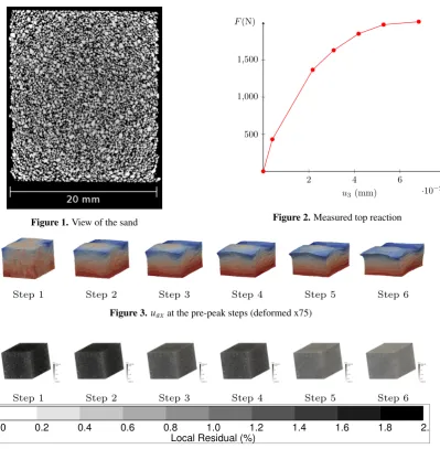
were excluded from the images because of the artifacts induced by the plates. A grayscale image of the tested 222

cemented sand is displayed in Figure1. During the test, the reaction is measured at the top of the sample. It is 223

plotted in Figure2. The first 6 steps (non-broken sample) are situated before the peak of the loading curve. 224

3.2. DVC and error estimation 225

The displacement fields at these different stages were calculated using a 3D-digital image correlation (DVC) 226

software named Ufreckles, developed by LaMCos (see Réthoréet al.[4]). A finite element continuum method is 227

used to calculate the displacement field with a non-linear least square error minimization method. The chosen 228

element size is near 0.5 mm. The final region of interest is 20.0_×22.4_×15.8 mm3. The top of the sample has been 229

excluded. The DVC is performed on a parallepipedic mesh composed of around 470,000 degrees of freedom. 230

The DVC showed that the pre-peak displacement field is extremely non-homogeneous as shown in Figure3. The 231

pre-peak noise is relatively homogeneous (Figure4). The noise is more predominant at the first steps where the 232

displacement is really small and thus the DVC reconstruction was more complicated. The test showed a complex 233

and rich behavior of the material tested with namely a non-homogeneous displacement field and pre-peak strain 234

bifurcations. The experimental data are very suited for testing the ability of a given model to predict such 235

Figure 1.View of the sand

2 4 6

·10−2 500

1,000 1,500

u3(mm) F(N)

Figure 2.Measured top reaction

Step 1 Step 2 Step 3 Step 4 Step 5 Step 6

Figure 3.uaxat the pre-peak steps (deformed x75)

Step 1 Step 2 Step 3 Step 4 Step 5 Step 6

0.0 0.2 0.4 0.6 0.8 1.0 1.2 1.4 1.6 1.8 2.0

Local Residual (%)

Figure 4.Noise at the pre-peak step (max: 2%)

3.3. Building the reduced experimental basis 237

As precised in the data pruning procedure, the experimental displacement and strain snapshot matrices are 238

computed. The attention is drawn to the fact that the studied test has not a lot of time steps (Nt=7) and the 239

experimental mesh is not that big. The DVC matricesQuandQεare respectively 474,405×7 and 1,774,080×14.

240

If the truncated SVD is applied on these matrices, only 6 modes are extracted for the displacement and 13 for 241

strain. As the number of time steps is rather small, the use of empirical modes does not reduce the size of the 242

experimental data, as stated before. 243

In other words, the experimental data are not suited for the dimensionality reduction. This method is 244

efficient on matrices with numerous columns and rather few lines, whereas tomographic data tend to have the 245

exact opposite : few columns (time steps) and a lot of lines (degrees of freedom). 246

3.4. RED after DVC on the specimen 247

The building procedure has three main inputs: 248

• The empirical modesVuandVε.

249

• TheKparameter for K-SWIM (Algorithm1). 250

During the test, the loading curve was measured at the top of the sample. In order to compare computed 252

and measured reactions for model assessment, the elements at the top of the mesh are considered as a ZOI. In the 253

remaining,Ω+is one layer of elements aroundΩu_∪Ω_ε∪Ωuser. 254

The RED was determined varying the numberKof selected lines in the K-SWIM Algorithm. Its influence is 255

assessed in Figure5. ForK=1, the standard DEIM algorithm selects very few degrees of freedom. Most of the 256

RED is actually the ZOI. This is due to the relatively low number of modes contained in the reduced basis (only 257

6). This apparent issue can be overcome by selecting more lines during the K-SWIM algorithm. When increasing 258

K, the number of degrees of freedom linearly rises. The attention is drawn on the fact that the resultant RED 259

forK=25 orK=50 are discontinuous, as it is usually the case when using hyper-reduction methods. The newly

260

selected zones are situated in the sheared regions. 261

(a)K=1 (b)K=25 (c)K=50

Nd=47,382 (10% ofΩ) Nd=73,911 (15.6% ofΩ) Nd=98,064 (20.5% ofΩ)

Figure 5.Influence ofKin the K-SWIM algorithm

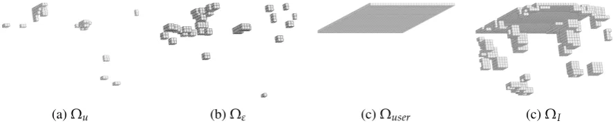
The final RED selected was the one computed withK=25(around 15.6% of the total domainΩ). It is 262

displayed in Figure5b. The reduced domain construction is analyzed in Figure6where the subdomainsΩu,Ω_ε, 263

ΩuserandΩ_Iare displayed. 264

(a)Ωu (b)Ω_ε (c)Ωuser (c)Ω_I

Figure 6.Different subdomains for the selected RED forK=25

A summary of the different matrix sizes at each step is displayed in Table1. As stated before, it’s clear that 265

for this kind of data, the PCA analysis does not reduce significantly the memory usage. The hyper-reduction 266

scheme used allowed to save up to 85% of the memory space for the illustrating example. 267

Experimental Data Empirical Modes Pruned data

Qu 474405×7 Vexpu 474405×6 Vexpu 73911×6

bexpu 6×7 bexpu 6×7

Memory saved 15% 85%

Experiments

Image acquisition

DIC/DVC

Data pruning Model reduced basis

H2_ROM

predictions

Cost Function

Optimized parametersµ∗

FEM calculations on Ω withµ∗

H2_ROM

prediction validated

Validatedµ∗ Parameter sensibility study

Initial guess

Updateµ

f

aexp_,η bexp

u Vexpu RED

µ0

Qmodel u

Vmodelu

bmodel_(µ)

No

Yes

Yes

No

Figure 7.Flowchart of the FEMU-H2ROM

4. Finite Element Model Updating-H2ROM 268

4.1. Assessing the relevance of the pruned data 269

In this section, the relevance of the pruned data for further usage is discussed. The data extracted from 270

computed tomography can have various purposes. This paper focuses on its use for model calibration, and is 271

illustrated with thein-situcompressive test of a resin bonded sand presented in the previous section. The main 272

aim of this part is to prove that a reduced integration domain computed thanks to a model free procedure is 273

relevant to assess or calibrate an arbitrary constitutive model. 274

It is supposed here that the inputs of the present section are: 275

• The mesh of the total experimental domainΩ; 276

• The mesh of the reduced experimental domainΩexp_R ; 277

• The reduced basis of the displacement on the RED and the corresponding reduced coordinatesVexpu and 278

bexpu ; 279

• The relevant boundary conditions; 280

• The probability distributions of shear strain onΩandΩexp_F . 281

The model used for the illustrating example is a constitutive elastoplastic model withmunknown parameters 282

to calibrate. The procedure employed is a Finite Element Model Updating (FEMU) technique, coupled with an 283

hybrid hyper-reduction method for the solution of approximate balance equations. The use of such method is 284

straightforward as the input data are actually hyper-reduced. This approach is termed FEMU-H2ROM. 285

The FEMU-H2ROM method is resumed in the flowchart of the Figure7. The blue part concerns the data pruning 286

q

p

p

p

_p

₍₁₊

_b

₎

f(b= 0) f(b >0)

Figure 8.Yield surfaces in the(p,q)plane

4.2. Constitutive model MC-CASM 288

4.2.1. Presentation 289

The resin-bonded sand behavior is modeled with a relatively simple constitutive model based on the 290

Cemented Clay and Sand Model (C-CASM). It consists in the extension of the Clay And Sand Model developed 291

by Yu [34] for unbonded sand and clay to bonded geomaterials within the framework developed by Gens and 292

Nova [35]. The C-CASM has been extensively described in Rioset al.[36]. The Modified Cemented Clay And 293

Sand Model (MC-CASM) presented here has some modifications of the C-CASM: 294

• Addition of a damage law whose equation is phenomenological (based on cycled compressive tests); 295

• The hardening law of the bonding parameterbis different: a first hardening precedes the softening. It is 296

supposed here that the polyurethane resin goes through a first hardening before breaking. 297

It is supposed here that the yield function was previously calibrated with standard laboratory tests. The 298

calibration concerns the parameters involved in the different damage and hardening laws that can be more difficult 299

to assess with macroscopic loading curves. In the continuation of the paper, the equivalent von Mises stress will 300

be denotedqand the mean pressurep. The MC-CASM equations are summarized hereafter. 301

4.2.2. Yield function 302

The yield function, f, of the constitutive model is defined by: 303

f(σ;pc,b) =

_q

M(p+pt)

n + 1

lnrln

_p

+pt

pc(1+b) +pt

(33)

M,r, andnare constant parameters that control the shape of the yield function.pcis the preconsolidation

pressure, that is to say the maximum yield pressure during an isotropic compressive test (see Roscoeet al.[37]). bis the bounding parameter modeling the amplification of the yield surface due to intergranular bonding. ptis the traction resistance of the soil defined by Gens and Nova [35] as:

pt=αbpc (34)

Whereαis a constant parameter modeling the influence of the binder on the traction resistance. The yield 304

function is supposed to be calibrated. This means thatM,r,n,αand the initial values ofpcandbare known. 305

The yield surfaces of the unbonded (blue) and bonded sand (red) are plotted in Figure8. 306

4.2.3. Hardening and damage laws 307

The model has two hardening variables: the preconsolidation pressurepcand the bonding parameterb. The evolution ofpcis directly controlled by the incremental plastic volumetric strainε˙pv, whereasbrelies on a plastic strain damage measureh:

˙ pc

pc =µ1ε˙

p

v (35)

˙

The incremental value ofhis defined as a weighting of the effects of the incremental plastic shear strain and the incremental plastic volumetric strain:

˙

h=µ2|ε˙ps|+µ3|ε˙pv| (37)

The model also includes a damage law whose formulation is purely phenomenological:

E=E0(1−D) (38)

D=µ4hµ5 (39)

The hardening and damage laws providem=7 unknown parameters to calibrate. 308

4.3. Calibration protocol by using the hybrid hyper-reduction method 309

The FEMU-H2ROM is preceded by an off-line phase similar to an unsupervised machine learning phase. It 310

consists in building the empirical reduced basisVthat is mandatory to set up the hybrid hyper-reduced equations. 311

It is similar to the first step of the data pruning method: a snapshot matrix is constructed based on simulations 312

and experimental results (and not on experiments only). 313

The starting point of the off-line phase is to assess the parameter sensibilities of the model starting from an 314

initial guessµ0={µ0₁, . . . ,µ0_m}. This guess can come from a previous calibration, or a calibration done using 315

macroscopic force-displacement curves of standard tests without predicting strain localization. 316

The off-line calculations are performed on the full domainΩand thus can be time consuming. The boundary 317

conditions are the experimental displacements taken from the computed tomography imposed at the top and 318

the bottom of the sample. The displacement field is not imposed inside the sample because one of the aims of 319

the model is to correctly capture the strain localization appearing inside the sample during the test, under the 320

constraint of balance equations. Imposing the displacement field inside the specimen gives less balance equation 321

to fulfill.mcalculations are made onΩ. Attention is drawn on the fact that these calculations can be done in 322

parallel. Only the displacement snapshot matrices are needed. A total ofm+1independent calculations are 323

performed: 324

• One initial calculation whereµ=µ0, which givesQu(µ0); 325

• mparameters sensibility calculations whereµ=µi ={µ0₁, . . . ,µ0_i +δµ0_i, . . . ,µ0_m}, which giveQu(µi) 326

fori=1, . . . ,m 327

Once done, these calculations are restricted to the reduced experimental domainΩexp_R . They are denoted

Qu(µi)fori=0, . . . ,m. All these results have to be aggregated in one snapshot matrixXbefore the computation of the empirical modesV. Instead of concatenating them+1matrices into one, a Derivative Extended Proper Orthogonal Decomposition (DEPOD) method is used (see Schmidtet al.[38]). This approach has been validated in previous works on model calibration with hyper-reduction Ryckelynck and Missoum Benziane [39]. This allows to capture the effects of each parameter variation.

X= [αVexp_u bexpu ,Qu(µ0), kQu(µ

0_)k

2kQu(µ1)−Qu(µ0)k(Qu(

µ1)−Qu(µ0)), . . . , kQu(µ0)k 2kQu(µm)−Qu(µ0)k

(Qu(µm)−Qu(µ0))] (40)

The first termαVexp_u bexpu corresponds to the pruned experimental data. It is weighted by a custom parameter 328

αthat enables to give more impact to the experimental fluctuations in the empirical modes. The finite element 329

methods tends to smooth these fluctuations thus provoking a certain loss of information. 330

Empirical modes depending on the factorαare displayed in Figure9. Forα=0, that is to say without 331

experimental data in the bulk, the empirical modes have strong fluctuations only at the top and the bottom of 332

the specimen, where the experimental boundary conditions are imposed. This can be explained by the natural 333

smoothing that ensures the finite element method with rather elliptic equations. Increasing the importance of the 334

modes (α=10) the last empirical mode is roughly smooth: this is due to the POD algorithm that filters the data. 336

In the sequel, we chooseα=1. The experimental data are as important as simulation data related to FE balance 337

equations. 338

α

= 0

α

= 1

α

= 10

First mode

Second mode

Third mode

Last mode

Figure 9._kukof the DEPOD modes depending onα

Once V is available, the hybrid reduced basis VH can be defined. Then, the experimental reduced coordinates are projected on the empirical reduced basis to be compared during the optimization loop:

b

bexp= (VH)TVexpu b exp

u (41)

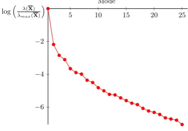
For the proposed example, there is a fast decay of the singular value (see Figure10whereePODis set to 339

10−4_{). When this decay is not sufficient to provide a small number of empirical modes, we refer the reader to}

340

Ghavamianet al.[40], Peherstorferet al.[41] and Haasdonket al.[42] to cluster the data in order to divide the 341

time interval and construct local reduced basis in time. 342

5 10 15 20 25

−6 −4 −2

Mode log λ(X)

λmax(X)

Figure 10.Singular values ofXverifyingλ(X)>ePODλmax(X)

4.4. Discussion on Dirichlet boundary conditions 343

After the data pruning, experimental data are available in allΩexp_R . When displacements are constrained to 344

follow the experimental data, we loose FE balance equations. The following property helps to discuss about the 345

Dirichlet boundary conditions. 346

Theorem 5. Ifα>0,etol=0and the experimental dataQ ex

u fulfill the FE equations onΩexR with the following additional Dirichlet boundary conditions:

and if both hybrid hyper-reduced equations and FE equations onΩex_R are unique, then the solution of the 347

hybrid hyper-reduced equation is the exact projection of the experimental data on the empirical reduced basis 348

bR(µ) = [(VTQex_u)T,0T_R]T, withkQex_u −V VTQex_u k=0. 349

Proof. Let’s consider a linear elastic FE problem. If Qexu fulfills the FE equations onΩexR, with additional Dirichlet boundary conditions, then:

aFE(tj,µ) =Qexu [:,j] j=1 . . .M

and

K[F?, :]aFE−c[F?] =0

Ifα>0andetol =0, then

aFE(tj,µ) =V bFE(tj,µ) j=1 . . .M,

with

bFE(tj,µ) =VTQex_u [:,j] j=1 . . .M

Then

K[F?, :]V bFE(tj,µ)−c[F?] =0 j=1 . . .M

and

(VH[F?, :])TK[F?, :]V bFE(tj,µ)−(VH[F?, :])Tc[F?] =0 j=1 . . .M

SobR(µ) = [(bFE(tj,µ))T,0T_R]Tis the unique solution of the hybrid hyper-reduced equations, and the exact 350

projection of the restrained FE solution. 351

The last property does not imply that imposingaFE(tj,µ)[I] = Qexu[I,j]as a boundary condition to 352

degrees of freedom in_I is the best way to fulfill FE balance equations. In fact, with the additional boundary 353

conditions on_I, the maximum of available FE equations is card(F?_{). The Property4means that if the empirical} 354

reduced basis is exact, then all theNd FE balance equations are fulfilled inΩ. In a sense, in the proposed 355

calibration protocol, we better trust in FE balance equations than in experimental data. Accurate FE balance 356

equations can be obtained by a convenient mesh ofΩ, although noise is always present in experimental data. 357

4.5. Cost function and parameters updating 358

In the optimization loop, a given set of parametersµis assessed. The H2ROM calculations provide the 359

reduced coordinates associated with the empirical basis previously determined on the RED denotedbR(µ). The 360

top reactionFcomp(µ)is also calculated as the average axial stress in the ZOI. 361

In the example, the cost function evaluates two scales of error: the microscale error between experimental and 362

computed reduced coordinates and the macroscale error between the measured and computed top reactions. 363

These error functions are respectively denotedχ2u(µ)andχ2_F(µ). 364

The microscale error is defined as:

χ2_u(µ) =kbR(µ)−bbexpk2_Ωexp R

(43)

The choice of the norm is user-dependent. The inverse covariance matrix of the displacement is the best norm for a Gaussian noise according to Tarantola [43], Kaipio and Somersalo [44] for a Bayesian framework. However, in this present study, to keep the treated problem rather simple, this error function is chosen:

χ2_u(µ) = (bR(µ)−bbexp)T(bR(µ)−bbexp) (44)

The macroscale error is defined as:

χ2_F(µ) =kFcomp(µ)−Fexpk2_Ωexp F

where Ωexp_F is the top of the sample, where the experimental load was measured. The experimental load measurements are supposed uncorrelated and their variance is denoted byσ2_F. In a Bayesian framework, for a Gaussian noise corrupting the load measurements [21], the previous equation can be written as:

χ2_F(µ) = 1

Ntσ_F2{F comp₍

µ)−Fexp}T{Fcomp(µ)−Fexp} (46)

For the the optimization loop, the final objective function is a weighted sum of the two previous sub-objective functions:

χ2(µ) =cuχ2u(µ) +cFχ2_F(µ) (47)

wherecuandcFare the weights. They can be chosen to balance the two cost functions or to privilege one scale 365

to another. In the illustrating example, the cost function is balanced. A classical Levenberg-Marquardt algorithm 366

is employed for the minimization of the error function and the update of the parameters vectorµ. 367

4.6. Model calibration and FEM validation 368

The optimization loop took 53 iterations. The speed ratio between FEM calculations and H2ROM predictions 369

is around 70. Moreover the H2ROM predictions only needed around 3% of the FEM calculation memory cost. 370

The H2ROM predictions converge way more easily than the FEM calculations. The problem simulated in the 371

optimization loop is a displacement imposed problem. The use of the reduced basis to predict the displacement 372

field facilitates drastically the convergence. That explains also the important speed-up time that does not come 373

only from the reduction of the integration domain. 374

Figure11displays the experimental and the computed top reactions (initial and optimized). At the end of the 375

optimization loop, it is mandatory to assess the relevance of the H2ROM prediction. The FEMU-H2ROM is 376

dependent on the initial guessµ0. This input determines the relevance of the reduced basis of the model after the 377

parameters sensibility study and the DEPOD analysis. During the model updating, the parameters set can be 378

too different from the initial guess. As a consequence, the empirical reduced basisVHmay not be accurate and 379

the H2ROM predictions will not be admissible. That is to say that the discrepancy between hyper reduced and 380

Finite Element calculations may not be negligible. That’s why the optimized parameters setµ∗must be validated 381

with FEM calculations on the full domainΩ. It is worth noting that if the experimental data are included in the 382

DEPOD, the final H2ROM prediction should be close to the experiments. 383

In a similar manner to the optimization loop, an error function between both calculations can be defined focusing 384

on the microscale (displacement error) and macroscale (top reactions differences). 385

Concerning the microscale, the discrepancy is only computed in the RED, as H2ROM predictions are only made 386

on this domain and cannot be reconstructed in the full domain with this particular approach. 387

r2_u(µ∗) =kaH 2_ROM

(µ∗)−aFE(µ∗)k2_Ωexp F

(48)

=aH2ROM(µ∗)−aFE(µ∗)

T

aH2ROM(µ∗)−aFE(µ∗)

(49)

In the same manner, the macroscale discrepancy is:

r2_F(µ∗) =kFH 2_ROM

(µ∗)−FFE(µ∗)k2_Ωexp F

(50)

=FH2ROM(µ∗)−FFE(µ∗)

T

FH2ROM(µ∗)−FFE(µ∗)

(51)

The microscale and macroscale errors should not exceed a few percents of the FEM calculations. In Figure11 388

the FEM top reaction is plotted in orange. It is clear that its value is extremely close to the one computed thanks 389

to H2ROM. The error is around 1% at each step. 390

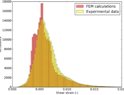
This final verification is purely numerical. If the H2ROM predictions are validated, it is advised to analyze deeper 391

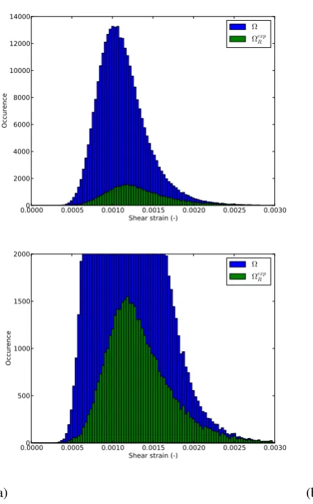
the RED. In the illustrating example, the computed and measured shear strain distributions were compared. The 393

analysis is summarized in the histograms displayed in Figure12for the last pre-peak step. The discrepancy 394

between computed and measured distributions was considered here as satisfying. 395

In the case of notable differences between H2ROM prediction and FEM calculations, or between FEM 396

calculations and experiment, the FEMU-H2ROM is not validated. Two solutions are possible to overcome this 397

issue: 398

1. Perform again the whole parameters sensibility study withµ0 = µ∗. This implies to do mparallel 399

calculations again. 400

2. Concatenate the previously determined matrix Xfrom Equation 40 withQu(µ∗)and perform a new 401

truncated SVD to determine ultimately an enriched reduced basisVH. No new FEM calculations are 402

needed. 403

The first solution should be performed in the case of strong differences between H2ROM prediction and FEM 404

calculations. The second option "only" costs a FEM calculation. It is also possible to modify the optimization 405

loop to include regularly FEM-H2ROM comparison and enrichVHincrementally. 406

1 2 3 4 5 6

·10−2

500 1,000 1,500

u3(mm)

F(N)

Experiment

µ0 µ∗ FEM verification

Figure 11.Result of the H2ROM optimization

5. Discussion 407

5.1. Limitations of the pruning procedure 408

The present paper focused on DVC sets and not on the images themselves. They are known to be as-well 409

particularly heavy and perhaps more problematic than the DVC data. The pruning procedure considers that 410

they can be deleted. Actually, it can be problematic. For instance, new DVC algorithm could improve the 411

determination of the displacement field (for example for complex problems involving cracks). 412

The images could be pruned too, in the sense that the only the pixels of the images inside the determined RED 413

can be conserved. However, we preconize to store only the reduced DVC data when the data storage is an issue. 414

In the case of non homogeneous materials, the data concerning the inhomogeneity outside the RED must be 415

saved as well. 416

5.2. A posteriori study of the RED 417

An a posteriori study of the determined RED was performed. The present discussion will focus on the 418

shear strain distributions inside the whole domainΩand the REDΩexp_R for the illustrating example. It would 419

be preferable that the pruning procedure stores in the RED the most different configurations. The shear strain 420

distributions in the whole domain and in the RED might be different (not the same mean value for example). The 421

Figures13(a) and14(a) present the shear strain distributions at the first and last pre-peak step. It appears that 422

the statistical distribution of the shear strain inside the RED is not the same than the one inside the full domain. 423

Nevertheless, zooms at both histograms in Figures13(b) and14(b) reveal that the extremum values of the shear 424

strain are conserved. One can see that the RED contains nearly all the elements where the shear is maximal. 425

Even if the proposed procedure is model-free, it is intimately linked with the mechanics of solids: it will store 426

preferably the data that is mechanically more relevant. For strain localization phenomenon, it is the most sheared 427

zone. The proposed method is not statistical: it induces actually a sampling bias. 428

6. Conclusion 429

The present paper proposed a pruning data procedure for DVC data that is model free and versatile. The 430

K-SWIM algorithm, through its parameterK, enables the user to define the size of the stored data. 431

The resultant data can still be used afterwards for calibration for instance. The use of hybrid hyper-reduction is 432

particularly suitable for the pruned data as it enables a non-negligible reduction of memory and time costs in the 433

FEMU optimization loop. The FEMU-H2ROM method is thus a new way to use massive DVC data for deeper 434

mechanical studies. 435

Acknowledgments 436

The authors would like to acknowledge the Agence Nationale pour la Recherche for their financial support 437

for the FIMALIPO project. 438

References 439

440

1. van Ooijen, P.M.A.; Broekema, A.; Oudkerk, M. Use of a Thin-Section Archive and Enterprise 3-Dimensional

441

Software for Long-Term Storage of Thin-Slice CT Data Sets—A Reviewers’ Response.Journal of Digital Imaging

442

2008,21, 188–192. doi:10.1007/s10278-007-9041-8.

443

2. Pan, D. A tutorial on MPEG/audio compression. IEEE MultiMedia1995,2, 60–74. doi:10.1109/93.388209.

444

3. Cioaca, A.; Sandu, A. Low-rank approximations for computing observation impact in 4D-Var data assimilation.

445

Computers and Mathematics with Applications2014,67, 2112 – 2126. Efficient Algorithms for Large Scale Scientific

446

Computations, doi:https://doi.org/10.1016/j.camwa.2014.01.024.

447

4. Réthoré, J.; Roux, S.; Hild, F. From pictures to extended finite elements: extended digital image correlation (X-DIC).

448

Comptes Rendus Mécanique2007,335, 131 – 137. doi:http://dx.doi.org/10.1016/j.crme.2007.02.003.

0.0000 0.0005 0.0010 0.0015 0.0020 0.0025 0.0030 Shear strain (-)

0 2000 4000 6000 8000 10000 12000 14000

Occur

ence

Ω Ωexp

R

0.0000 0.0005 0.0010 0.0015 0.0020 0.0025 0.0030 Shear strain (-)

0 500 1000 1500 2000

Occur

ence

Ω Ωexp

R

(a) (b)

Figure 13.Shear strain distributions in the whole domain and in the RED at the first step

5. Rojanaarpa, T.; Kataeva, I. Density-Based Data Pruning Method for Deep Reinforcement Learning. 2016

450

15th IEEE International Conference on Machine Learning and Applications (ICMLA), 2016, pp. 266–271.

451

doi:10.1109/ICMLA.2016.0051.

452

6. Hu, Y.; Chen, H.; Li, G.; Li, H.; Xu, R.; Li, J. A statistical training data cleaning strategy for the PCA-based chiller

453

sensor fault detection, diagnosis and data reconstruction method. Energy and Buildings2016,112, 270 – 278.

454

doi:https://doi.org/10.1016/j.enbuild.2015.11.066.

455

7. Hong, Y.; Kwong, S.; Chang, Y.; Ren, Q. Unsupervised data pruning for clustering of noisy data. Knowledge-Based

456

Systems2008,21, 612–616. doi:{10.1016/j.knosys.2008.03.052}.

457

8. Kavanagh, K.T.; Clough, R.W. Finite element applications in the characterization of elastic solids. International

458

Journal of Solids and Structures1971,7, 11 – 23. doi:https://doi.org/10.1016/0020-7683(71)90015-1.

459

9. Kavanagh, K.T. Extension of classical experimental techniques for characterizing composite-material behavior.

460

Experimental Mechanics1972,12, 50–56. doi:10.1007/BF02320791.

461

10. Ienny, P.; Caro-Bretelle, A.S.; Pagnacco, E. Identification from measurements of mechanical fields by finite

462

element model updating strategies. European Journal of Computational Mechanics 2009, 18, 353–376,

463

[https://www.tandfonline.com/doi/pdf/10.3166/ejcm.18.353-376]. doi:10.3166/ejcm.18.353-376.

464

11. Lecompte, D.; Smits, A.; Sol, H.; Vantomme, J.; Hemelrijck, D.V. Mixed numerical–experimental technique for

465

orthotropic parameter identification using biaxial tensile tests on cruciform specimens. International Journal of

466

Solids and Structures2007,44, 1643 – 1656. doi:https://doi.org/10.1016/j.ijsolstr.2006.06.050.

467

12. Molimard, J.; Le Riche, R.; Vautrin, A.; Lee, J.R. Identification of the four orthotropic plate stiffnesses using a single

468

open-hole tensile test.Experimental Mechanics2005,45, 404–411. doi:10.1007/BF02427987.

0.000 0.005 0.010 0.015 0.020 Shear strain (-)

0 2000 4000 6000 8000 10000 12000 14000 16000

Occur

ence

Ω Ωexp

R

0.000 0.005 0.010 0.015 0.020 Shear strain (-)

0 500 1000 1500 2000

Occur

ence

Ω Ωexp

R

(a) (b)

Figure 14.Shear strain distributions in the whole domain and in the RED at the last step

13. Meijer, R.; Douven, L.F.A.; Oomens, C.W.J. Characterisation of Anisotropic and Non-linear Behaviour of

470

Human Skin In Vivo. Computer Methods in Biomechanics and Biomedical Engineering 1999, 2, 13–27,

471

[https://doi.org/10.1080/10255849908907975]. PMID: 11264815, doi:10.1080/10255849908907975.

472

14. Bruno, L. Mechanical characterization of composite materials by optical techniques: A review. Optics

473

and Lasers in Engineering 2018, 104, 192 – 203. Optical Tools for Metrology, Imaging and Diagnostics,

474

doi:https://doi.org/10.1016/j.optlaseng.2017.06.016.

475

15. Mahnken, R.; Stein, E. A unified approach for parameter identification of inelastic material models in the frame

476

of the finite element method. Computer Methods in Applied Mechanics and Engineering1996,136, 225 – 258.

477

doi:https://doi.org/10.1016/0045-7825(96)00991-7.

478

16. Forestier, R.; Massoni, E.; Chastel, Y. Estimation of constitutive parameters using an inverse method coupled

479

to a 3D finite element software. Journal of Materials Processing Technology 2002, 125-126, 594 – 601.

480

doi:https://doi.org/10.1016/S0924-0136(02)00406-5.

481

17. Giton, M.; Caro-Bretelle, A.S.; Ienny, P. Hyperelastic Behaviour Identification by a Forward Problem Resolution:

482

Application to a Tear Test of a Silicone-Rubber. Strain2006,42, 291–297.

483

18. Cugnoni, J.; Botsis, J.; Janczak-Rusch, J. Size and Constraining Effects in Lead-Free Solder Joints. Advanced

484

Engineering Materials2006,8, 184–191. doi:10.1002/adem.200400236.

485

19. Latourte, F.; Chrysochoos, A.; Pagano, S.; Wattrisse, B. Elastoplastic behavior identification for heterogeneous

486

loadings and materials. Experimental Mechanics2008,48, 435–449. doi:10.1007/s11340-007-9088-y.

487

20. Padmanabhan, S.; Hubner, J.P.; Kumar, A.V.; Ifju, P.G. Load and Boundary Condition Calibration Using Full-field

488

Strain Measurement. Experimental Mechanics2006,46, 569–578. doi:10.1007/s11340-006-8708-2.