Eliminating Variables in Boolean Equation Systems
Bjørn Møller Greve1,2, H˚avard Raddum2, Gunnar Fløystad3, and Øyvind Ytrehus2
1 Norwegian Defence Research Establishment 2
Simula@UiB
3 Dept. of Mathematics, UiB
Abstract. Systems of Boolean equations of low degree arise in a natural way when analyzing block ciphers. The cipher’s round functions relate the secret key to auxiliary variables that are introduced by each successive round. In algebraic cryptanalysis, the attacker attempts to solve the resulting equation system in order to extract the secret key. In this paper we study algorithms for eliminating the auxiliary variables from these systems of Boolean equations. It is known that elimination of variables in general increases the degree of the equations involved. In order to contain computational complexity and storage complexity, we present two new algorithms for performing elimination while bounding the degree at 3, which is the lowest possible for elimination. Further we show that the new algorithms are related to the well knownXLalgorithm. We apply the algorithms to a downscaled version of the LowMC cipher and to a toy cipher based on the Prince cipher, and report on experimental results pertaining to these examples.
1
Introduction
A block cipher encryption algorithmEK(P) =Ctakes a fixed length plaintextP and a secret key K as inputs, and produces a ciphertext C. The encryption usually consists of iterating a round function, which in turn is made up by suitable linear and nonlinear transformations. In a known plaintext attack, bothP andC are known to the cryptanalyst, who wants to find the secret keyK. Ciphers defined overGF(2) can be described as a system of multivariate Boolean equations of degree 2. These equations relate the bits of the secret keyKand newauxiliary variables that arise due to the round functions via the knownP andC. Solving this system of equations with respect to the secret keyKis known asalgebraic cryptanalysis. The approach in this paper is to iteratively eliminate the auxiliary variables that arise in an initial such system of Boolean equations. At each iteration, the elimination step converts a current system of polynomial equations F in the variablesx1, . . . , xninto a set of new equationsF0 inx2, . . . , xn, so that the solution set ofF0is the projection of the solution set ofF ontox2, . . . , xn. We propose two algorithms for the elimination step: L−Elim∗() (a variant of XL with bounded degree) and eliminate∗() (a new algorithm based on the mathematical framework developed in this paper), where ∗ ∈ {A,B} denotes one of two variants. In both algorithms the polynomial degree is limited to 3 at all times in order to contain computational complexity and storage complexity. The highlight of the paper is Theorem 11, where we show that the more efficient algorithm eliminateA() produces the same output as L−ElimA(). In addition we show that by applying a few extra tricks, the B-variants of the algorithms can produce more equations than the A-variants.
The paper is structured as follows. Section 2 describes the problem, the notation, and previous results. The foundation for elimination techniques over the Boolean ring is developed in Section 3. The new algorithms,L−Elim∗() and eliminate∗(), are presented in Section 4 along with discus-sions of complexity and information loss. In Section 5 we report on experimental results of the new algorithms when applied to reduced block ciphers: A reduced version of the LowMC cipher, and a
2
Notation and Preliminaries
Consider the quotient ring of Boolean polynomials innvariables. We denote the ring by
B[1, n] =F2[x1, . . . , xn]/(x2i +xi|i= 1, . . . , n). A monomial is a productxi1· · ·xiδ ofδdistinct (because x
2=x) variables, where δis the degree of this monomial. The degree of a polynomial
p=X s
ms
where thems’s are distinct monomials, is the maximum degree over the monomials inp. Given a set of polynomial equations F ={fi(x1, . . . , xn) = 0|i= 1, . . . , m}, our objective is to find its set of solutions in the spaceFn2. The approach we take in this paper is to solve the system of equations by eliminating variables.
In the following we assume without loss of generality that we eliminate variables in the order x1, x2, . . . , xn. Consider the projection which omits the first coordinate:
π1:Fn2 →F n−1 2
(a1, a2, . . . , an)7→(a2, . . . , an),
and denote by B[2, n] the ring of Boolean polynomials wherex1 has been omitted. We may in a similar fashion consider a sequence ofkprojections
Fn2 →F n−1
2 → · · · →F n−k 2 , where the i’th projection is denoted πi : Fn2−i+1 → F
n−i
2 for 1≤ i ≤ k. We denote the ring of Boolean functions where we omit the sequence of variablesx1, . . . , xk as B[k+ 1, n].
2.1 Systems of Boolean equations and ideals
The polynomials inF ={f1, . . . , fm}generate an idealI= (f1, . . . , fm) =I(F) in the ringB[1, n]. LetZ(I) denote the zero set of this ideal, i.e, the set of points
Z(I) ={a∈Fn
2|f(a) = 0 for everyf ∈I}.
Lemma 1 Let f, g be Boolean functions inB[1, n]. Then the following ideals are equal:
(f, g) = (f g+f+g).
Proof. Clearly (f, g) ⊇ (f g+f +g). Note that also Z(f, g) = Z(f g+f +g), since it is easy to check that f(a) = g(a) = 0 if and only if f(a)g(a) +f(a) +g(a) = 0. Thus the zero set Z(f)⊇Z(f g+f+g). This in turn means that the Boolean functionf is a multipleh(f g+f+g) for some other Boolean function h, and similarly forg. Thus
(f, g)⊇(f g+f+g)⊇(f, g),
which shows that these ideals are equal.
Corollary 2 Any ideal I = (f1, . . . , fm) in B[1, n] is a principal ideal. More precisely I = (f)
where
f = 1 + m
Y
i=1
Proof. Let I = (f1, . . . , fm). By Lemma 1 this is equal to the ideal (f1f2+f1+f2, f3, . . . , fm), with one generator less. We may continue the process for the remaining generators providing us in the end withI= (f), where
f = 1 + m
Y
i=1
(fi+ 1).
Corollary 3 For two ideals in B[1, n] we have I ⊇J if and only if Z(I)⊆ Z(J). In particular
I=J if and only if Z(I) =Z(J).
Proof. By Corollary 2 we have I = (f) andJ = (g), where f and g are the respective principal generators. Clearly if (f)⊇(g) thenZ(g) containsZ(f). If the zero set of gcontains the zero set off, theng =f hfor some polynomialh. Hence (f)⊇(g).
Now given an ideal I ⊂ B[1, n], our aim is to find the ideal I2 ⊂B[2, n] such that Z(I2) = π1(Z(I)). More generally, when eliminating more variables we aim to find the ideal Ik+1⊂B[k+ 1, n], such thatZ(Ik+1) =πk◦(· · · ◦(π1(Z(I)))). Since the complexity of the polynomials can grow very quickly when eliminating variables, we would rather want to compute an ideal J, as large as possible given computational restrictions, which is contained inIk+1.
If we can find solutions to Z(J) contained in Fn2−k we can then check if they lift to solutions in Z(I) contained in Fn
2, by sequentially lifting the solutions backwards with respect to each projection. Let us first describe precisely the idealIk+1whose zero set is the sequence of projections πk◦(· · · ◦(π1(Z(I)))). This corresponds to what is known as theelimination ideal I∩B[k+ 1, n]. Lemma 4 Let Ik+1 ⊆ B[k+ 1, n] be the ideal of all Boolean functions vanishing on πk ◦(· · · ◦ (π1(Z(I)))). ThenIk+1=I∩B[k+ 1, n].
Proof. We show this for the case when eliminating one variable, the general case follows in a similar manner. ClearlyI2⊇I∩B[2, n]. Conversely letf ∈B[2, n] vanish onπ1(Z(I)). Thenf must also vanish onZ(I), wheref is regarded as a member of the extended ringB[1, n]. Thereforef ∈Iby Corollary 3.
A standard technique for computing elimination ideals is to use Gr¨obner bases, which eliminate onemonomial at the time. Computing Gr¨obner bases is computationally heavy because the degrees of the polynomials grow rapidly over the iterations. To deal with this problem we propose two algorithms which attempt to limit the degrees of polynomials that arise. Our solution is to not use all elements during elimination, butdiscard high degree polynomials and only keep the low-degree ones.We denote an ideal where the degree is restricted to someδ byJδ, whereasJ∞ means that
we allowall degrees.
The benefit from our solution is that the elimination process gives us an algorithm with much lower complexity, at the cost of the following two disadvantages:
1. Discarding polynomials of degree> δgives an idealJδthat is only contained in the elimination ideal J∞ = I∩B[j+ 1, n] for 1 < j ≤ k. It follows that Z(Jδ) of the eliminated system contains all the projected solutions of the original set of equations, but it will also contain “false” solutions which will not fit the ideal I when lifted back to Fn2, regardless of which values we assign to the eliminated variables.
It is important to note thatnot discarding any polynomials will provide only the true solutions to the set where variables have been eliminated, which then can be lifted back to the solutions of the initial ideal I. The drawback of this approach is that we must be able to handle arbitrarily large polynomials, i.e high computational complexity.
Thus there is a tradeoff between the maximum degree δ allowed, and the proximity between the “practical” idealJδ and the true elimination ideal I∩B[k+ 1, n].
In this paper we limit the degree toδ= 3, and we therefore consider the two sets
F3={f13, . . . , fr33}, F2={f12, . . . , fr22}
of polynomials, where the fi3’s all have degree 3 and the fi2’s have degree≤2. Furthermore, the polynomials inF3andF2together generate the idealI= (F3, F2). We use the notationFxi1, F
i x1, (i = 2,3) to distinguish disjoint subsets that contain (resp. do not contain) any monomial with the variablex1. In the following sections we are going to develop the mathematical framework for computing idealsI2, . . . , Ik such thatIj⊆I∩B[j+ 1, n] starting from the idealI, and such that the generators for eachIj has degree≤3.
3
Elimination Techniques
Several methods for solving systems of Boolean equations based on various approaches have been suggested. In [5] and [6] the authors introduce the XL and XSL algorithms, respectively. The basic idea is to multiply equations with enough monomials to re-linearize the whole system of Boolean equations. Our approach can be viewed as a specialized generalization of this approach. By this we mean that since we bound the degree at≤3, the quadratic equations will only be multiplied with linear monomials. The aim is to squeeze out as many quadratic and cubic polynomials which in turn can be used to solve the system of Boolean equations. Furthermore, we note that the elimination aspect is not considered in the XL and XSL approaches.
Our objective is to find as many polynomials in the idealIgenerated byF2andF3as possible,
computing only with polynomials of degrees ≤3. This limits both the storage and computational complexity. Our approach to solve the system of equations
fiδ = 0, δ= 2,3 andi= 1, . . . , rδ
is to eliminate variables so that we find degree ≤ 3 polynomials in Ik, in smaller and smaller Boolean ringsB[k+ 1, n]. We introduce the algorithms for doing this in Section 4.
LetF = (f1, . . . , fm) be a set of Boolean functions inB[1, n] of degree≤3, and denote byhFi the vector space spanned by the polynomials inF, where each monomial is regarded as a coordinate. Let L = {1, x1, . . . , xn} consist of the constant and linear functions in B[1, n], such that hLi is the vector space spanned by the Boolean polynomials of degree ≤ 1. For the set of quadratic polynomialsF2, we denote the productLF2 as the set of all productslgwhere l∈Landg∈F2. Then it suffices to eliminate variables from the vector space hF3∪LF2i. For convenience we let the setF = (f1, . . . , fm) be the set of cubic polynomials generated byF3∪LF2.
Hence, as part of the variable elimination process, it will be necessary to split a set of poly-nomials according to different criteria. Two procedures, Algorithm 6:SplitV ariable() and Algo-rithm 7:SplitDeg2/3() are described in Appendix A.SplitV ariable(F, x1) splits a setF of polyno-mials into the subsetsFx1, Fx1, whereFx1 only has polynomials that containx1 andFx1 consists of all polynomials not containingx1.SplitDeg2/3(F) splits a setFof polynomials into the subsets F2, F3, where polynomials inF2 are quadratic, and polynomials inF3 have degree 3.
These two procedures can essentially be implemented in terms of row reduction on the incidence matrices of F, where the monomials (i. e. columns of the matrices) are ordered lexicographically and by degree, respectively. More details are provided in Appendix A.
a2x1+b2 be two polynomials inB[1, n], where the variablex1 has been factored out. Then the polynomialsajandbj are inB[2, n]. In order to find the resultant, form the 2×2 Sylvester matrix off1andf2with respect to x1
Syl(f1, f2, x1) =
a1a2 b1 b2
Theresultant off1 and f2 with respect to x1 is then simply the determinant of this matrix, and hence a polynomial inB[2, n]:
Res(f1, f2, x1) = det(Syl(f1, f2, x1)) =a1b2+a2b1
We note that Res(f1, f2, x1) = a2f1+a1f2, which means that the resultant is indeed in the ideal generated byf1andf2. Moreover, Res(f1, f2, x1) is in the elimination idealI2and when both fi’s are quadratic, then theai’s are linear so the degree of the resultant Res(f1, f2, x1) is≤3.
This observation gives hope for computational purposes, since 2×2 determinants are easy to compute and cubic polynomials can be handled by a computer, also for the number of variables nwe encounter in cryptanalysis of block ciphers. Note that one resultant computation eliminates all monomials containing the targeted variable, and not only the leading term, as in Gr¨obner basis computations.
For an idealI(F) = (f1, . . . , fm)⊆B[1, n] generated by a setF of Boolean polynomials, we can compute the resultant of every pair of polynomials Res(fi, fj;x1), which in turn gives us the ideal of resultants:
Res2(F;x1) = (Res(fi, fj;x1)|1≤i < j≤m).
It is easy to show that the ideal of resultants is contained in the elimination idealI(F)∩B[2, n], but this inclusion is in general strict. To close the gap we need the following ideal:
Definition 5 Let I(F) = (f1, . . . , fm) ⊆B[1, n], and write each fi as fi = aix1+bi, where x1
does not occur inai orbi. We define the coefficient constraintideal:
Co2(F) = (b1(a1+ 1), b2(a2+ 1), . . . , bm(am+ 1)).
Note that the degrees of the generators of Co2(F) have the same degrees as the generators of the resultant ideal. In the case whenI(F) consists of quadratic polynomials, the generators of Co2(F) will be polynomials of degree≤3. The zero set of this ideal lies in the projection of the zero set ofI(F) onto Fn2−1.
Lemma 6 Z(Co2(F))⊇π1(Z(I(F))).
Proof. Note that a point p∈ F2n−1 is not in the zero setZ(Co2(F)) only if for some i we have ai(p) = 0 andbi(p) = 1. But then for both the two liftings ofptoF2n:p0= (0,p) andp1= (1,p) we have fi(pj) = 1. Thereforep∈/ π1(Z(I(F))), and so we must haveZ(Co2(F))⊇π1(Z(I(F))). By Lemmas 4 and 6, the coefficient constraint ideal is in the elimination ideal. We can now use this ideal to describe the full elimination ideal, which turns out to be generated exactly by Res2(F) and Co2(F).
Theorem 7 Let I(F) = (f1, . . . , fm)⊆B[1, n] be an ideal generated by a setF of Boolean
poly-nomials. Then
I(F)∩B[2, n] =I(Res2(F), Co2(F)).
Proof. By Lemma 4 we have
We know that
I(F)∩B[2, n]⊇I(Res2(F),Co2(F)), which implies that
π1(Z(I(F))) =Z(I(F)∩B[2, n])⊆Z(Res2(F))∩Z(Co2(F)).
Conversely, let a pointp∈Fn2−1in the right hand side above be given. Then it has two liftings to points inFn2:p0= (0,p) andp1= (1,p). Letfi=x1ai+bibe an element inF. Sincepvanishes on Co2(F), the following are the possible values for the terms infiwhen applied to the liftingpj.
aibix1 0 0 0 0 0 1 1 0 0 1 1 1
Note that Co2(F) excludes ai(p) and bi(p) from taking the values 0,1. Since pvanishes on the resultant ideal, there cannot be two fi and fj such that ai(p), bi(p) takes values 1,0 and aj(p), bj(p) takes values 1,1, since in that case the resultant aibj +ajbi does not vanish. This means that the values ofai(p), bi(p) are eitheri) All 0,0 or 1,0, orii) All 0,0 or 1,1. In case i), the liftingp0is in the zero setZ(I(F)). In caseii) the liftingp1is in the zero set ofZ(I(F)). This shows that Z(Res2(F))∩Z(Co2(F)) lifts to Z(I(F)), which means that
π1(Z(I(F))) =Z(I(F)∩B[2, n])⊇Z(Res2(F))∩Z(Co2(F)) as desired.
Note that since we limit the degree to≤3, we only compute resultants and coefficient constraints with respect to the setF2consisting of quadratic Boolean functions. The process of producing the resultants and the polynomials of the coefficient constraints of the set F2 with respect to the variablex1 is described in Algorithm 1.
Algorithm 1RandC(F2 x1, x1) In: F2
x1= (f
2
1, . . . , fr22) set of quadratic polynomials inB[1, n]
Out: SetR of cubic polynomials whereπ1(Z(Fx21)) =Z(R) andx16∈R fi2=aix1+bifor 1≤i≤r2
R=∅
for(fi2, fj2)∈Fx21×F
2
x1, f
2
i 6=fj2 do R←R∪ {aibj+ajbi}
end for forfi2∈F
2
x1 do
R←R∪ {bi(ai+ 1)}
end for ReturnR
Corollary 8 ForI(F) = (f1, . . . , fm) inB[1, n], then
I(F)∩B[k+ 1, n] =I(Resk+1(F), Cok+1(F)).
It is important to note that Corollary 8 is only valid if we allow the degrees to grow with each elimination, but including the coefficient constraints solve the problem with the resultant only being a subset of the elimination ideal. This enables us to actually compute the elimination ideal not depending on any monomial order. Moreover, one could find the elimination ideal by successively eliminatingx1, . . . , xk using Corollary 8 by the following algorithm:
1. F1=F,
2. F2= generators of Res2(F1) +Co2(F1), 3. F3= generators of Res3(F2) +Co3(F2), 4. · · ·
However, applying this strategy in practice leads to problems due to the growing degrees of the resultants and coefficient constraints with each elimination. In fact if the fi’s have degree d, the degrees of the resultants and the coefficient constraints have degree 2d−1. With many variables the size of the polynomials and the number of monomials quickly become too large for a computer to work with. This is the reason why we limit the degree at ≤3, enabling us to deal with these complexity issues.
4
Elimination Algorithms
4.1 The LG-algorithm A
In the following we are going to apply the procedure A. below as a building block in order to produce as many polynomials of degree≤3 as we can when eliminating variables from the setsF3 andF2.
A.We compute two setsFx21 andFx31 of quadratic and cubic polynomials inB[2, n], that satisfy
hFx21∪F 3 x1i=hF
3∪LF2i ∩B[2, n]. This gives a new pair of setsF3
x1andF 2
x1, but now in the smaller ringB[2, n]. This procedure can be continued givingF3
x1,x2,...,xk in smaller and smaller Boolean ringsB[k+ 1, n]. The computation
of F2 x1 andF
3
x1 is the main objective of our algorithm. In Algorithm 2 we show how we perform this procedure in L-ElimA.
Algorithm 2L−ElimA(F3, F2, x 1)
In: F3= (f13, . . . , fr33) set of cubic polynomials inB[1, n],F
2
= (f12, . . . , fr22) set of quadratic polynomials inB[1, n], andx1the variable to be eliminated fromF3 andF2
Out: SetFx31 of cubic polynomials and setF
2
x1 of quadratic polynomials, wherex16∈F
2
x1∪F
3
x1 L={1, x1, . . . , xn}
F∗←F3∪L·F2
F2, F3←SplitDeg2/3(F∗) F2
x1, F
2
x1←SplitV ariable(F
2, x 1)
Fx31, F
3
x1←SplitV ariable(F
3
, x1)
ReturnF3
x1, F
2
x1
Remark 9 Computational complexity:The heaviest step inL−ElimAis the call toSplitDeg2/3(). This procedure does Gauss elimination on O(n3) columns in a matrix with O(n3) rows. In total
Remark 10 Algorithm 2 is related to the XL and XLS algorithm [5],[6], where we restrict the al-gorithm here by only multiplying with linear Boolean monomialsL. However, our approach contains the aspect of elimination of variables which is not considered in XL-type algorithms.
Next, we proceed to develop a more efficient algorithm. In fact, the next construction optimizes the elimination approach by showing that we do not need to multiply with all variables as done in L−ElimA().
4.2 Main elimination algorithm A
Motivated by Algorithm 2, we aim in a similar fashion to produce more polynomials of degree≤3 for the setsF3, F2, but in a more efficient way. We use resultants, coefficient constraints and some other steps to be detailed below. The ensuing algorithmeliminateA() is presented in Algorithm 3. The inputs toeliminateA() are setsF3andF2, of polynomials of degree 3 and 2 respectively. These sets will be modified in the algorithm to only include polynomials without x1, the variable to be eliminated. We also want the sets to be as large as possible, but of course only with linearly independent polynomials.
eliminateA() starts by splittingF2 into subsetsF2
x1 containingx1 andF 2
x1 not containingx1, usingSplitV ariable(). These sets are first used to increaseF3, by addingx
1Fx21 and (x1+ 1)F 2 x1 to F3. Note that we multiplyF2with only one variable (x
1, to be eliminated), and not all of Las in L−ElimA(). This leads to much lower space complexity ineliminateA(), since theFx31 computed here is much smaller than the one output from L−ElimA(). Then we split F3 into subsets Fx31 containingx1 andFx31 not containingx1, usingSplitV ariable().
Next,Fx31 is normalized (see Algorithm 8:N ormalize() in Appendix B) withF 2
x1 as basis. This removes many of the degree 3 monomials containingx1 inFx31, and if a polynomial on the special formf∞=x1+g(x2, . . . , xn) is found inFx21 all degree 2 monomialsx1xi will be eliminated from F3
x1. The output ofN ormalize() isF 3,norm x1 andF
3,norm
x1 , and we joinF 3,norm x1 toF
3 x1. Now we compute resultants and coefficient constraints from the set F2
x1, creating a setR of cubic polynomials inB[2, n] by using Algorithm 1RandC(). This produces as many polynomials withoutx1as possible. All of these are added toFx31 and we remove potentially linearly dependent polynomials inF3
x1 such that
Fx3 1 :=F
3 x1∪F
3,norm
x1 ∪R (1)
The two new setsF2 x1, F
3
x1 in B[2, n], neither containingx1, are returned fromeliminateA(), as described in Algorithm 3. In the following we show that in fact the output ofeliminateA() and L−ElimA() is the same.
Theorem 11 LetF2, F3be the input toeliminateA(). LetFx21 be the subset ofF2 not containing
x1 and letFx31 be the defined as in (1). Then
hFx31∪Lx1F 2 x1i=hF
3
∪LF2i ∩B[2, n].
Proof. The fact thathF3∪LF2i ∩B[2, n]⊇ hF3
x1∪Lx1F 2
x1iis obvious from the construction. To prove the converse, if a polynomialf2∈F2
x1has leading termx1xiwe denote the polynomial as f2 =f2
i =aix1+bi. Similarly, if it has leading term x1 we denote it by f2 =f∞2. With this
notation we letI⊆ {2, . . . , n}∪{∞}be the index set of these polynomials, such thatF2 x1={f
2 i}i∈I. LetF2
x1 be{f 2
j}j∈J for some index setJ such that J∩I=∅.
Letpbe a polynomial inhF3∪LF2i ∩B[2, n]. We can then write p=f3+fx3
1+f 3 x1 where f3 ∈F3, f3
x1 ∈ hL·F 2
x1i, andf 3
x1 ∈ hL·F 2
x1i. The goal is to subtract from pthe terms in F3
x1∪Lx1F 2
x1 which is produced according to (1). In the end we will show that we are left with p= 0, which proves thatpis originally inhF3
Withpas above we can find index sets I0, I1⊆I and J0 ⊆J, and K ⊆ {2, . . . , n} ×I such that
fx31 =
X
i∈I0
(x1+ 1)fi2+
X
i∈I1 fi2+
X
(k,i)∈K xkfi2,
fx31 = X j∈J0
x1fj2+f 30,
wheref30∈ h{1, x
2, . . . , xn}Fx21i=hLx1·F 2 x1i.
By the normalization we may write the following part ofp:
f3+X i∈I0
(x1+ 1)fi2+
X
j∈J0 x1fj2
as
fx3,norm1 + X (k,i)∈K0
xkfi2+f 3,norm x1
for some index set K0 with all k ∈ {2, . . . , n}, and where fx3,norm1 ∈ hF 3,norm
x1 i and f 3,norm
x1 ∈
hF3 x1∪F
3,norm
x1 i. So we have
p=fx3,norm1 +X i∈I1
fi2+ X (k,i)∈K00
xjfi2+f
30+f3,norm
x1 (2)
whereK00=K∪K0.
Now we consider the terms above withf2
2. Supposex2f22occurs in the sum on the right. Note thatx1x2 is not inp(sincep∈B[2, n]), and not infx3,norm1 (since it is 3-normal). Sox1x2inx2f
2 2 must cancel against x1x2 in f22. Thenf22+x2f22= (x2+ 1)f22occurs. Now
(x2+ 1)f22= (a2+ 1)f22+ smaller terms thanx1x2.
We now subtract (a2+ 1)f22= (a2+ 1)b2 (which is inB[2, n]) from both sides of (2). So its new left side is:
p:=p−(a2+ 1)f22, and the new right side of (2) will contain neitherf2
2 norx2f22(while it may containxjf22forj≥3). It follows that the left side of (2) above will not containx2f22.
If now in the new equation (2),x2f32occurs, thenx1x2x3must cancel againstx3f22(sincex2f22 does not occur any more on the right side of (2), andx1x2x3 does not occur inpnor infx3,norm1 ). We substract the resultant a2f32+a3f22from both sides of (2). So its new left side is:
p:=p−(a2f32+a3f22).
Then neitherx2f22norx2f32will occur anymore on the right side of (2). In this way we continue and no term x2fi2 with 2 ≤i ≤n will occur in the right side of (2). If x2f∞2 occurs, then x1x2 must cancel against the same term inf2
2. We then subtract the corresponding resultant from both sides of (2) and its new left side is:
p:=p−(a2f∞2 +f22).
Now we continue and remove terms x3fi2 from the right side of (2). Then we remove terms x4fi2 and so on. Considering the pin (2), we then get that modulo Co2 and Res2 we can write it as
p=fx3,norm1 +X j∈I0
fj2+f30+fx3,norm 1
for some I0 ⊆I. If f2
2 occurs, the termsx1x2 could not cancel against anything infx3,norm1 , thus f2
2 does not occur. Iff32 occurs, the term x1x3 could not cancel against anyting on the right side above, sincef22does not occur. Hencef32 does not occur. In this way we could continue and in the end get
p=fx3,norm1 +f30+fx3,norm 1 .
But then clearlyf3,norm
x1 equals 0. Thus modulohCo2∪Res2ithe originalpis inhLx1·F 2 x1i+hF
3 x1∪ Fx3,norm
1 i. This proves the Theorem.
Corollary 12 Let Lx1,...,xk = {1, xk+1, . . . xn} and F
3
x1,...,xk, F
2
x1,...,xk be the result of applying
eliminateA()ktimes to the input setsF3,F2. Then
hF3∪LF2i ∩B[k+ 1, n] =hFx31,...,xk∪Lx1,...,xkF
2 x1,...,xki.
Proof. Given a sequence of variables x1, x2, . . . , xk to be eliminated. Then applying Theorem 11 onx1gives ushF3∪LF2i ∩B[2, n] =hFx31∪Lx1F
2
x1i. Applying Theorem 11 on the next variable x2onhFx31∪Lx1F
2
x1iwe get
hF3∪LF2i ∩B[3, n] =hFx3
1∪Lx1F 2
x1i ∩B[3, n] =hF 3
x1,x2∪Lx1,x2F 2 x1,x2i.
Continuing this way for the rest of the variables to be eliminated, it follows thathF3∪LF2i ∩ B[k, n] =hF3
x1,...,xk∪Lx1,...,xkF
2
x1,...,xkias desired.
Algorithm 3eliminateA(F3, F2, x1)
In: F3 = (f13, . . . , fr33) set of cubic polynomials in B,F
2
= (f12, . . . , fr22) set of quadratic polynomials in B,x1 variable to be eliminated fromF3 andF2
Out: SetF3
x1 of cubic polynomials wherex16∈F
3
x1 and setF
2
x1 of quadratic polynomials wherex16∈F
2
x1
F2
x1, F
2
x1←SplitV ariable(F
2, x
1) .Thefi2∈Fx21 will have unique leading monomials containingx1 F3←(x1+ 1)Fx21∪x1F
2
x1∪F
3
F3
x1, F
3
x1←SplitV ariable(F
3, x 1)
Fx3,norm 1 , F
3,norm
x1 ←N ormalize(F
3
x1, F
2
x1) F3
x1 ←R and C(F
2
x1, x1)∪F
3
x1∪F
3,norm x1 ReturnFx31, F
2
x1
The output comprises setsFx21 and Fx31 of polynomials of degree 2 and 3 respectively. These are nontrivial polynomials of the same degree as the input polynomials and neither set contains the variablex1. The two sets satisfyhFx21, F
3
For complexity, we haveO(n3) andO(n2) monomials and polynomials inFx31 andFx21, respec-tively. If there were more polynomials than monomials we could solve the system by re-linearization. Hence the space complexity of the algorithm is storingO(n6) monomials which in practice is storing
O(n6) bits.
The time complexity for normalization can be estimated as follows: There are at mostndifferent f2
i in Fx1. For each of the O(n
3) polynomials in F3, there may be n monomials containing the leading term off2
i. Each of these needs to be cancelled by adding a multiple offi2, costingO(n3) bit operations. The total worst-case complexity for the normalization step is thenO(n×n3×n×n3) =
O(n8) bit operations.
The time complexity for computing resultants and coefficient constraints can be estimated similarly to also beO(n8).
The time complexity for SplitV ariable() can be estimated as follows. In the worst case, we have input sizeO(n3) in both polynomials and monomials, so the matrices constructed are of size
O(n3)× O(n3). In the Gaussian reduction we need to create 0’s under leading 1’s inO(n2) columns (those corresponding to monomialsx1xaxb), and this costsO(n3×n3×n2) =O(n8) bit operations. Hence the total time complexity for Algorithm 3 isO(n8) bit operations.
4.3 Extensions of L-ElimA(): L-ElimB()
In this section we improveL−ElimA() andeliminateA() by adding the heuristic procedure B, in the following form:
B.It is conceivable that the vector spacehF3∪LF2icontains more relations of degree≤2, beyond the ones in F2. Hence we may improve on procedure A, by adding a search for more quadratic relations. This can be done by ordering the monomials such that the degree 3 monomials are bigger than the degree 2 monomials, and then split the system into degree 2 and 3 polynomials by calling SplitDeg2/3().
LetF2,(1)=F2, and computehF3∪LF2,(1)i. CallingSplitDeg2/3(F3∪LF2,(1)) returns new sets F3 and F2,(2). If hF2,(2)i is strictly larger than the space hF2,(1)i, we continue to compute splitDeg2/3(F3∪LF2,(2)), repeating the process.
We continue such computations until hF2,(i)i = hF2,(i−1)i for some i. Setting F2 := F2,(i) we can then continue with A, which is the elimination step. In the case that SplitDeg2/3() on F3∪LF2,(1)does not yield any new quadratic polynomials, we proceed directly to the elimination step.
Remark 13 The advantage of adding B: Finding new quadratic polynomials allows to ”com-pute with monomials of degree ≥4 by computing with monomials of degree ≤3”. More precisely, suppose we find a new quadratic polynomial h, so:
h=f3+X i
lifi2
where f3∈F3 and theli ∈L andfi2∈F
2, and his not inhF2i. Thenhcan again be multiplied
with a linear polynomial and added tohF3∪LF2i to form
f30+lh+X i
l0if 2 i =f
30+lf3
+X
i
llifi2+
X
i li0f
2 i
The terms inlf3andll
ifi2 are generally of degree4, but they cancel so in reality we only work
with polynomials of degree≤3.
Algorithm 4L−ElimB(F3, F2, x 1)
In: F3 = (f13, . . . , fr33) set of cubic polynomials in B[1, n],F
2,(1)
= F2 = (f12, . . . , fr22) set of quadratic polynomials inB[1, n],L={1, x1, . . . , xn}andx1 the variable to be eliminated fromF3 andF2
Out: SetFx31 of cubic polynomials and setF
2
x1 of quadratic polynomials, wherex16∈F
2
x1∪F
3
x1
F∗←F3∪L·F2,(1) .procedureA
F2,(2), F3 ←SplitDeg2/3(F∗) i= 2
whilehF2,(i)i 6=hF2,(i−1)ido .procedureB F∗←F3∪L·F2,(i)
F2,(i+1), F3←SplitDeg2/3(F∗) i=i+ 1
end while F2=F2,(i)
Fx21, F
2
x1←SplitV ariable(F
2
, x1) .procedureA
Fx31, F
3
x1←SplitV ariable(F
3
, x1)
ReturnF3
x1F
2
x1
Remark 14 Computational complexity: Part B includes a while loop where we have to call
SplitDeg2/3() every time. A naive implementation would require an additionalO(n9) operations
per loop iteration. However, since SplitDeg2/3() in the loop is called on the argument F∗ which may change only by a little for each loop iteration, it is possible that more efficient algorithms exist.
4.4 Extensions of main elimination algorithm eliminateA(): eliminateB()
In a similar manner as in the previous subsection, we can also extendeliminateA() toeliminateB(). Instead of usingBonhF3∪LF2i, we useBon the setF3,norm
x1 which is the output of the normal-ization step, and the setFx31:=Fx31∪Fx3,norm
1 ∪R (SeeeliminateA() and equation (1)). LetF2
x1 :=F 2,(1) x1 and F
2 x1 :=F
2,(1)
x1 . Calling SplitDeg2/3() onF 3,norm x1 and F
3
x1, returns the sets F3
x1, F 2,(2) x1 , F
3
x1, and F 2,(2)
x1 . If either of the spaces hF 2,(2) x1 i, hF
2,(2)
x1 i are strictly larger than the spaces hFx2,(1)1 iand hF
2,(1)
x1 i, we continue to compute normal forms, resultants and coefficient constraints as ineliminateA(), repeating the process.
We continue these computations untilhFx2,(i)1 i=hF 2,(i−1)
x1 iand hF 2,(i) x1 i=hF
2,(i−1)
x1 ifor some i≥1. SettingF2
x1 :=F 2,(i) x1 andF
2 x1 :=F
2,(i)
x1 , we simply return the new setsF 3 x1 andF
2 x1. In the case thatSplitDeg2/3() onF3
x1, F 3
x1 does not yield any new quadratic polynomials, we proceed directly to SplitV ariable() on F3
x1, and return F 3
x1 and F 2
x1 as before. eliminateB() is described in Algorithm 5. Again the only difference betweeneliminateA() and eliminateB(), is the partial addition ofB.
The following summarizes the constructions we have done in this section.
1. We can eliminate variables in two different ways: By eitherL−ElimA(), or byeliminateA(). The latter algorithm has significantly lower complexity than the first, since we avoid to multiply withall variables in L.
2. We can produce extra polynomials of degree ≤ 2 by adding B to L−ElimA(), giving the algorithmL−ElimB().
3. We can produce extra polynomials of degree≤2 by adding a partial version ofBtoeliminateA(), yieldingeliminateB(), with significantly lower complexity thanL−ElimB().
4.5 Information loss
Algorithm 5eliminateB(F3, F2, x 1)
In: F3 = (f13, . . . , fr33) set of cubic polynomials inB,F
2,(1)
= (f12, . . . , fr22) set of quadratic polynomials inB,x1variable to be eliminated fromF3 andF2
Out: SetFx31 of cubic polynomials wherex16∈F
3
x1 and setF
2
x1 of quadratic polynomials wherex16∈F
2
x1
Fx21,(1), F
2,(1)
x1 ←SplitV ariable(F
2,(1)
, x1) .Thefi2∈F
2,(1)
x1 will have unique leading monomials containingx1
i= 1
whilehFx21,(i)i 6=hF
2,(i−1)
x1 iorhF
2,(i)
x1 i 6=hF
2,(i−1)
x1 ido .procedureB
F3←(x
1+ 1)Fx21∪x1F
2
x1∪F
3
F3,norm x1 , F
3,norm
x1 ←N ormalize(F
3, F2
x1) Fx31←R and C(F
2
x1, x1)
F2,(i+1), F3←SplitDeg2/3(Fx31,norm∪F
3,norm x1 ∪F
3
x1) Fx21,(i+1), F
2,(i+1)
x1 ←SplitV ariable(F
2,(i+1), x 1)
i=i+ 1 end while Fx31, F
3
x1←SplitV ariable(F
3
, x1)
F2
x1 =F
2,(i)
x1 ReturnFx31, F
2
x1
random variable that takes values x1, . . . , xM with probabilities pi = P(X = xi), i = 1, . . . , M. The (binary) entropy ofX is defined as
H(X) =−
M
X
i=1
pilog2pi. (3)
If X is uniformly distributed, i. e.pi = 1/M, i= 1, . . . , M, then H(X) = log2M. Given X and another random variable Y that assumes values y1, . . . , yM0, the conditional entropy of X given
that we observe thatY takes a specific value yis
H(X|Y =y) =−
M
X
i=1
P(X =xi|Y =y) log2P(X =xi|Y =y), (4)
and the information that we get aboutX by observingY =y isH(X)−H(X|Y =y).
The application of the concept of entropy in the context of this paper is as follows. A cryptan-alyst wishes to recover a secretk-bit keyK. A priori,K will be assumed to be drawn uniformly from the set of all keys, so H(K) =k. A setF of equations that K must satisfy will reduce the entropy ofK if not all possible key values satisfy all equations inF. HenceF containsinformation
about the secret keyK and we define
i(F) = Number of key bits−log2(Number of key values that satisfyF). (5) The iterative elimination algorithms described in this section produce sequences of equation sets F0, F1, F2, . . ., where Fj = Fx21,...,xj ∪F
3
x1,...,xj denotes the set of equations contained after
5
Experimental Results
We have implementedL−ElimB() andeliminateB() and done some experiments to see how they perform in practice. In this section we report on these experiments.
5.1 Reduced LowMC cipher
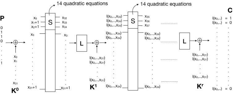
LowMC is a family of block ciphers proposed by Martin Albrecht et al. [1]. The cipher family is designed to minimize the number of AND-gates in the critical path of an encryption, while still being secure. The cipher itself is a normal SPN network, with each round consisting of an S-box layer, an affine transformation of the cipher block and addition with a round key. All round keys are produced as affine transformations of the user-selected key.
Two features of the LowMC ciphers are interesting with respect to algebraic cryptanalysis. First, the S-box used is as small as possible without having linear relations among the input and output bits. LowMC uses a 3×3 S-box, where the ANF of each output bit only contains one multiplication of input bits, making the three output polynomials of the S-box quadratic. We can search for other quadratic relations in the six input/output variables, and we then find 14 linearly independent quadratic polynomials.
Second, the S-boxes in one round do not cover the whole state, so a part of the cipher block is not affected by the S-box layer. The number of S-boxes to use in each round is a parameter that varies within the cipher family, and some variants are proposed with only one S-box per round.
The cipher parameters we have used for the reduced LowMC version of our experiments are:
– Block size: 24 bits – Key size: 32 bits – 1 S-box per round – 12 or 13 rounds
As will become clear below, the number of rounds is on the border of whenL−ElimB() and eliminateB() are successful in breaking the reduced cipher.
Constructing equation system. The attack is a known plaintext attack, where we assume we are given a plaintext/ciphertext pair and the task is to find the unknown key. We use the 14 quadratic polynomials describing the S-box as the base equations. The bits in the unknown key are assigned as the variables x0, . . . , x31, and the output bits from each S-box used in the cipher are the variables x32, . . .. All other operations in LowMC are linear, so the input and output bits of every S-box can be written as a linear combination of the variables defined and the constants from the plaintext.
Inserting the actual linear combination for each input/output bit of the S-box in one round will produce 14requations in total. These equations describe a LowMC encryption overrrounds. The initial number of variables is 32 + 3r, but this can be reduced by using the known ciphertext. The bits of the cipher block output from the last round are linear combinations of variables. These linear combinations are set to be equal to the known ciphertext bits, giving 24 linear equations that can be used to eliminate 24 variables by direct substitution. After this the final number of variables is 8 + 3r. See Fig. 1 for the equation setup.
Experimental results. The goal of our experiment is to try to eliminate all the variables xi for i ≥ 32, and find some polynomials of degree at most 3, only in variables representing the unknown user-selected key. If we are able to find at least one polynomial only in x0, . . . , x31 for one given plaintext/ciphertext pair, we can repeat for other known plaintext/ciphertext pairs and build up a set of equations that can be solved by re-linearization when the set has approximately
32 3
Fig. 1.Setup of equation system representing reduced LowMC. Alll(.)’s only indicate some linear combi-nation, and are not equal.
12 rounds:The system initially contains 44 variables and 168 quadratic equations.
We first useL−ElimB() to eliminate the 12 variables with highest indices. With this method we succeed in producing 1-2 cubic polynomial(s) only in key variables (some p/c-pairs produce 1, others produce 2 polynomials). The memory requirement is to store the 7560 polynomials we get after multiplying the quadratic equations with all terms in L.
Next we apply theeliminateB() algorithm on the same system. Initially the setF2 contains 168 polynomials and the set F3 is empty. As the algorithm proceeds, eliminating one variable at the time, the sizes of F3 and F2 change. The set F3 grows at first before starting to decrease before the last variables are eliminated, while the set F2 decreases at a steady pace during the 12 eliminations. The size ofF3 was never above 2000 polynomials, soeliminateB() has considerably less space complexity than L−ElimB(). The observed running time of the two methods were roughly the same, andeliminateB() produced the same polynomials asL−ElimB() in the end. Finally we generate 15 different systems using different p/c-pairs, to see how many indepen-dent polynomials in x0, . . . , x31 we get when collecting all outputs from the 15 systems together. The 15 systems collectively produced 20 polynomials in only key bits, of which 16 were linearly independent. So the hypotheses that we can produce many independent polynomials from different p/c-pairs seems to hold.
At this stage we noticed something unexpected. After doing Gaussian elimination on the 20 polynomials to check for linear dependencies, it turned out that we produced five linear polyno-mials in the unknown key variables. It therefore appears that the polynopolyno-mials produced from the elimination algorithm are not completely random, and that one may need much fewer polynomials than anticipated to actually find the values ofx0, . . . , x31.
13 rounds:The initial system contains 47 variables and 182 quadratic equations.
Neither L −ElimB() nor eliminateB() were able to find any cubic polynomials in only x0, . . . , x31 for any 13-round systems we tried. So for the reduced LowMC version we used, only up to 12 rounds may be attacked using our elimination techniques and bounding the degree to at most 3.
5.2 Toy Cipher
and a key addition. The same key is used in every round. For the elimination experiments reported here we use a 4-round version of the toy cipher.
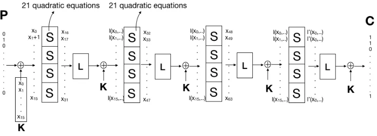
Constructing equation system. The equation system representing the toy cipher is constructed similarly to the reduced LowMC. The variables in the unknown key arex0, . . . , x15, and the output bits of every S-box, except for the last round, are variablesx16, . . . , x63. The inputs and outputs of every S-box can then be described as linear combinations of the variables we have defined, together with the constants in the known plaintext and ciphertext blocks. See Fig. 2 for the setup of the equations.
Each output bit of the PRINCE S-box has degree 3 when written as a polynomial of the input bits, but there exists 21 quadratic relations in input/output variables describing the S-box. The number of quadratic equations in the 4-round toy cipher is therefore 336, in the 64 variables x0, . . . , x63.
Fig. 2.Setup of equation system representing 4-round toy cipher. Alll(.)’s andl0(.)’s indicate some linear combination of variables.
Experimental results. When trying to eliminate all non-key variables x16, . . . , x63 from the system, neither L−ElimB() nor eliminateB() were able to find any cubic polynomial in only x0, . . . , x15.
We know that when runningeliminateB() we will throw away polynomials giving constraints on the solution space on the way, and hence introduce false solutions. WhenF3andF2become empty the whole space becomes the solution space, and we have lost all information about the possible solutions to the original equation system. It is interesting to measure how fast the information about the solutions we seek disappear, and this is what we have investigated for the toy cipher.
As in all algebraic cryptanalysis we are interested in finding the possible values for the secret key. In this case this means finding the values ofx0, . . . , x15. With only a 16-bit key it is possible to do exhaustive search, and check which key values that fit in any of the equation systems we get after eliminating some variables. The procedure we used for checking if one guessed key fits in a given system is as follows:
– Fixx0, . . . , x15 to the guessed value in the system
– Do Gauss elimination on the resulting system to produce linear equations – Use each linear equation found to eliminate one more variable
– If all variables get eliminated without producing any 1-polynomial, the guessed key fits – If we fail to produce linear equations in the Gauss elimination, it is undecided whether the
guessed key fits or not
We set up an elimination order where variables to be eliminated were distributed evenly throughout the system. That is, we do not eliminate the second variable from an S-box before all S-boxes have at least one variable eliminated. The exact elimination order used was
x36, x24, x52, x44, x20, x56, x40, x28, x60, x32, x16, x48, x18, x50, x34, x26, x58, x46, x54, x22, x62, x30, x38, x42, x47, x21, x49, x35, x29, x59, x41.
After eliminating these 31 variables, all keys fit in the system we have at that point. For each system we get along the way, we checked how many keys that fit in the given system. This gives a measure of how much information the system has about the unknown secret key we try to find. For a systemF, we usei(F) (5) that says how much information the system has about the key:
i(F) = 16−log2(# of keys that fit inF).
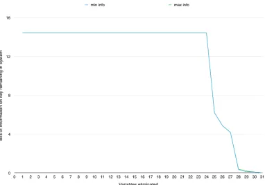
Denote the system we have after eliminatingvvariables asFv. For the plaintext/ciphertext pair we used there were three keys that fit in the initial system, so we havei(F0)≈14.42. We know that i(F) is a strictly non-increasing function for increasing v, because we can only lose information during elimination. Put another way, if the keyK fits inFv,K will also fit inFwforw > v. It is interesting to see what the rate of information loss is during elimination. Is the information loss gradual, or do we lose all information more suddenly? In Fig. 3 we have plotted the graph fori(Fv) for 0≤v≤31.
As we can see in Fig. 3, we can eliminate up to 24 of the 48 non-key variables in the system without losing any information on the possible keys. The three keys that fit in the original system are still the only ones that fit in F24. After that, all information on possible keys is lost rather quickly, and i(F31) = 0. Only in F27 and F28 did we run into some cases where it could not be decided whether a guessed key fits or not. This is barely visible in Fig. 3, where there is a tiny area where the true values ofi(F27) andi(F28) may lie.
We find this behavior interesting and a source for further study. We can look at it this way: It is possible to describe a cipher by quadratic equations inkkey variables andn−knon-key variables (i.e. constructed as in Figs. 1 and 2). Our experiment indicates that (at least sometimes) one can create a cubic equation system, with the same information on the key, with only k+ (n−k)/2 variables. In other words, there is a trade-off between degree and number of variables needed to describe a cipher. For the toy cipher, increasing the degree by one allows to cut the number of non-key variables in half to describe the same cipher.
6
Conclusions
In this paper we proposed two new algorithms for performing elimination of variables from systems of Boolean equations: L−Elim∗() which is essentially Gaussian elimination, and eliminate∗() which is more efficient and when suitably extended also more effective. We applied these algorithms in a known plaintext attack to two reduced versions of the LowMC cipher: 12 and 13 rounds with 24 bits block and 32 bits key. For the 12-round version the algorithms produces polynomials of degree 3 in only key variables, while in the 13-round example the algorithms fail to find any polynomials of degree 3 in only key variables.
We also applied the algorithms to a toy cipher for performing tests, where the proposed al-gorithms fails to find any polynomials of degree 3 in only key variables. Instead we extend the experiments by measuring how much information we lose about the key during elimination. Sur-prisingly, the experiments show that we can eliminate many auxiliary variables from the system of equations, without losing any information about the key. Another result of the experiments is that we lose information about the key rather quickly after a certain point in the elimination process. We conclude that there is a lot of future work to be done in this direction.
References
1. M. Albrecht, C. Rechberger, T. Schneider, T. Tiessen, M. Zohner.Ciphers for MPC and FHE, Euro-crypt 2015, LNCS 9056, pp. 430 – 454, Springer, 2015.
2. D.Cox, J.Little, D.O’Shea,Ideals, varieties and algorithms, Third edition, 2007 Springer Science and Business Media.
3. D.Cox, J.Little, D.O’SheaUsing Algebraic GeometryGTM 185, Springer Science and Business Media 2005.
4. Kipnis A., Shamir A.Cryptanalysis of the HFE Public Key Cryptosystem by Relinearization. Advances in Cryptology — CRYPTO’ 99. CRYPTO 1999. Lecture Notes in Computer Science, vol 1666, pp. 19 – 30. Springer, Berlin, Heidelberg 1999.
5. A. Shamir, J. Patarin, N. Courtois, A. Klimov, Efficient Algorithms for solving Overdefined Systems of Multivariate Polynomial Equations, Eurocrypt’2000, LNCS 1807, pp. 392 — 407, Springer 2000. 6. Courtois N.T., Pieprzyk J.Cryptanalysis of Block Ciphers with Overdefined Systems of Equations,
Ad-vances in Cryptology — ASIACRYPT 2002. ASIACRYPT 2002. Lecture Notes in Computer Science, vol 2501, pp. 267 – 287. Springer, Berlin, Heidelberg 2002
7. Murphy S., Robshaw M.J. Essential Algebraic Structure within the AES. Advances in Cryptology — CRYPTO 2002. CRYPTO 2002. Lecture Notes in Computer Science, vol 2442, pp. 1 – 16. Springer, Berlin, Heidelberg 2002
8. Biryukov A., De Canni`ere C.Block Ciphers and Systems of Quadratic Equations, Fast Software En-cryption, FSE 2003. Lecture Notes in Computer Science, vol 2887, pp. 274 – 289. Springer, Berlin, Heidelberg 2003
Appendix A: Monomial orders and splitting algorithms
Consider the vector spacehFi=hF3∪LF2iwhich is generated by the set of Boolean polynomials F3, F2. We can perform Gaussian reduction on this vector space with two different orders. In the Gaussian elimination we order the monomials such that the largest monomials are eliminated first.
A. The monomial order where x1-monomials are largest: hFi can be realised as a matrix A. Each row ofA corresponds to one polynomial inF3∪LF2, and each column corresponds to one monomial m. Moreover, the entry A[i, j] corresponds to the coefficient of the j’th monomial in the i’th polynomial. Whenx1-monomials are the largest, we consider the leftmost columns ofA to correspond to all monomials containing x1. Note that for the matrix A, we write A[i . . . j] to indicate the submatrix consisting of rowsithroughjofA. With a slight abuse of notation, we write x1∈m, x1∈f or x1∈Gto indicate thatx1 occurs in monomialm, polynomialf or polynomial set G.
When performing Gaussian elimination on A with this order, we can create polynomials in the span of F3∪LF2 that have 0’s in the leftmost columns. If there are enough polynomials in F3∪LF2, the lower rows ofA will then give a non-empty set of polynomialsF3
x1∪LF 2
x1 that do not contain thex1-variable. Note that the new setFx31∪LF
2 x1 ⊇F
3∪LF2∩B[2, n].
B.The order where higher-degree monomials are larger: It is conceivable that hFi=hF3∪LF2i contains more quadratic polynomials than just the ones inF2. These can be found if we order the monomials such that the degree 3 monomials are bigger than degree 2 monomials. We can then use Gaussian elimination on the matrix ArepresentinghFi=hF3∪LF2ito eliminate monomials of degree 3 and possibly produce more quadratic equations than there are originally inF2.
The algorithm for splitting polynomial sets into those containing x1 and those which do not containx1is given in Algorithm 6 below. The algorithm for splitting a set of degree 3 polynomials into degree 2 and 3 polynomials is given in Algorithm 7 below. We are going to use these orders in section 4 as building blocks for finding more quadratic and cubic polynomials when developing the elimination algorithms.
Algorithm 6SplitV ariable(F, x1)
In: F = (f1, . . . , fm) set of polynomials of degree≤3 inB[1, n]
Out: SetsFx1 andFx1 of polynomials such thathFi=hFx1∪Fx1i, x1∈Fx1 andx1 6∈Fx1
m= (m1, . . . , mc, mc+1, . . . , mt)←monomials occurring inF wherex1∈mifor 1≤i≤candx16∈mi
fori > c.
A←m×tmatrix where coefficient ofmjinfi is entryA[i, j]
Row-reduceAsuch that leading 1’s in rowsi≤rare in columnsj≤cand leading 1’s in rowsi > r are in columnsj > c.
Fx1 =A[1. . . r]mT Fx1 =A[r+ 1. . . t]m
T
ReturnFx1, Fx1
Appendix B: Normalizing Cubics with Respect to Quadratics
Algorithm 7SplitDeg2/3(F)
In: F = (f1, . . . , fm)⊆B[1, n] is set of polynomials of degree≤3.
Out: SetsF2of quadratic polynomials andF3of cubic polynomials such thathFi=hF2∪F3i.
m = (m1, . . . , mc, mc+1, . . . , mt) ← monomials occurring inF where deg(mi) = 3 for 1≤ i≤c and
deg(mi)≤2 fori > c.
A←m×tmatrix where coefficient ofmjinfi is entryA[i, j]
Row-reduceAsuch that leading 1’s in rowsi≤rare in columnsj≤cand leading 1’s in rowsi > r are in columnsj > c.
F2=A[1. . . r]mT F3=A[r+ 1. . . t]mT ReturnF2, F3
usually has a beneficial effect on both efficiency and information preservation. Moreover, the pro-cedure is a technical requirement for the proof of Theorem 11. Before giving the algorithm, we develop a mathematical foundation around the process of normalization.
Since we in this paper are considering the setsFx21 andF 3
x1, we normalize the polynomials in Fx31 with respect to the setF
2
x1 and the variablex1. With the orders on the monomials introduced in Section 2, it follows that any non-zero Boolean polynomial f3 ∈ B[1, n] of degree 3 has a
leading term. This is the largest monomial in f with respect to the given order. For a given set F2 ={f2
1, . . . , fr22} of quadratic polynomials with distinct leading terms, the polynomial f 3 is in
normal form with respect to the set F2
x1, if no monomial in f
3 is divisible by the leading term of any polynomial in F2
x1. A polynomial f
3 can be brought into a normal form f3,norm (not in general unique) by successively subtracting multiples of the polynomials inF2
x1. More specifically, we obtainf3,norm by the following procedure. Let
f3=mf3+ lower order terms, fi2=mf2
i + lower order terms,
and assume that mf2
i dividesmf3. Then we can writemf3 =qmfi2 where qis a monomial whose
set of variables is disjoint from that of mf2
i. We can now replace f
3 by f3+qf2
i, cancelling the term mf3 in the process. Doing this successively will eventually produce the normal form off3 with respect tof2
i, and performing this for all generators will eventually produce the normal form off3 with respect to the setF2
x1.
Note that there is a specific case that merits attention, namely when there is a polynomialf2 i in F2
x1 with leading termx1. Then this term is the only term in f 2
i involving the variablex1. To distinguish this polynomial, we denote it by
f∞2 =x1+h, h∈B[2, n]. Extra care is needed when F2
x1 contains f 2
∞ with leading term x1. The reason is that when following the procedure for making normal forms, we would remove every term in the polynomials ofFx31 containing the variablex1. This will also imply that we replacef3∈Fx31 byf
3+qf2
∞, where
q is a quadratic monomial. Then the newf3,norm in general will involve terms of degree 4, which we do not allow. However, we may still freely usef∞2 to remove allquadratic termsinf3containing x1. Hence, whenf∞2 is found in Fx21 there will be no quadratic monomials in F
3
x1 containing x1 after normalization. A normal form off3 using this procedure we call a 3-normal form, to signify that we do not do computations with monomials of degree≥4.
The complete algorithm for producing normal forms for a setF3
x1 of cubic polynomials using a set F2
x1 of quadratic polynomials as a basis, including possiblyf 2
Algorithm 8N ormalize(F3 x1, F
2 x1) In: F3
x1= (f
3
1, . . . , fr33) set of cubic polynomials inB[1, n],F
2
x1 = (f
2
1, . . . , fr22) set of quadratic polynomials inB[1, n] withmf2 unique leading term (in some order) infi2
Out: SetFx31,norm where no monomialm∈Fx31,normcontainsx1 and setFx31,normwhere each polynomial contains at least one monomial withx1
Fx3,norm 1 , F
3,norm x1 ← ∅ forf2∈Fx21 do
mf2 ←leading monomial inf2 if mf2=x1 then
d←2 else
d←3 end if
forf3∈Fx31 do
forall monomialsm∈f3,deg(m)≤d do if mf2 dividesmthen
f3←f3+ m mf2f
2
.eliminate monomial divisible bymf2 end if
end for end for end for forf3∈F3
x1 do if x1∈/f3 then
Fx3,norm 1 ←F
3,norm x1 ∪f
3
else F3,norm
x1 ←F
3,norm x1 ∪f
3
end if end for
ReturnFx31,norm, F