Physik-Department, Technische Universität München, James-Franck-Str. 1, 85748 Garching, Germany
Abstract.We discuss divergences of loop functions in thermal QCD and compute per-turbatively the Polyakov loop, the Polyakov loop correlator and the cyclic Wilson loop. We show how these functions get mixed under renormalization.
1 Thermal loop functions
Thermal loop functions are gauge invariant quantities that can be computed by lattice QCD and that are relevant for the dynamics of static sources in a thermal bath at a temperatureT [1] (for a review, see [2]). We will focus on three loop functions.
ThePolyakov loopaverage in a thermal ensemble at a temperatureT is defined as
P(T)|R≡
1 dRTr
LR, (1)
where R is the color representation:dA=N2−1,dF =N,Nis the number of colors, and
LR(x)=P exp
ig
1/T
0
dτA0(x, τ)
. (2)
The operator P stands for the path ordering of the color matrices. A graphical representation is in figure 1.
Figure 1.Polyakov loop.
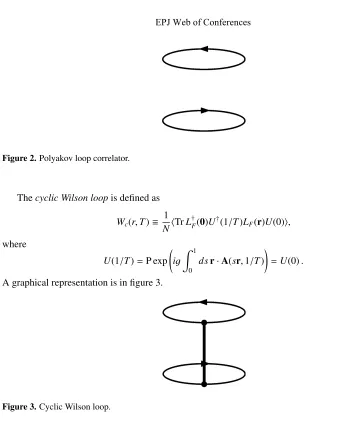
ThePolyakov loop correlatoris defined as
Pc(r,T)≡
1 N2TrL
†
F(0)TrLF(r), (3)
whereris the spatial separation of the two loops. A graphical representation is in figure 2.
Figure 2.Polyakov loop correlator.
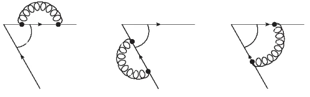
Thecyclic Wilson loopis defined as
Wc(r,T)≡
1 NTrL
†
F(0)U†(1/T)LF(r)U(0), (4)
where
U(1/T)=P exp
ig 1
0
dsr·A(sr,1/T)
=U(0). (5)
A graphical representation is in figure 3.
Figure 3.Cyclic Wilson loop.
1.1 Divergences
Loop functions are affected by divergences. These are ultraviolet divergences coming from regions where two or more vertices are contracted to one point. In the case of internal vertices, divergences are removed by charge renormalization. But for loop functions one also gets divergences from the contraction of line vertices along the contour. Thesuperficial degree of divergenceis given byω = 1−Nexat a smooth point andω =−Nexat a singular point, whereNexis the number of propagators connecting the contraction point to uncontracted vertices.
Three type of divergences related to line vertices are possible.
(1) All vertices are contracted to a smooth point, which leads to a linear divergence. Linear divergences are proportional to the length of the contour and can be removed by a mass term.
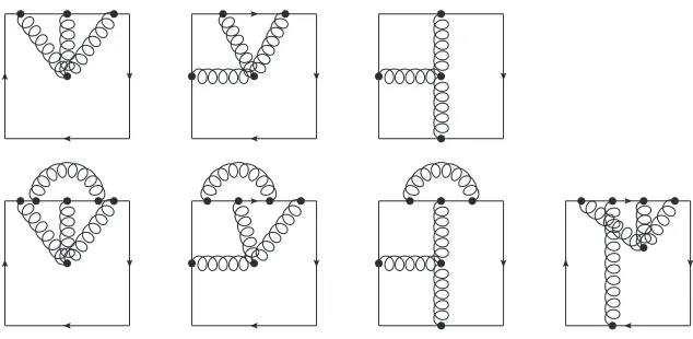
Figure 4.Contributions to a cusp divergence atO(αs).
A special case is the case of a non-cyclic (time extension smaller than 1/T) rectangular Wilson loop. This has four right-angled cusps. The multiplicative renormalization constant in the MS-scheme is at one loop
Z=exp−2CFαsμ−2ε/(π¯ε)
, 1/¯ε≡1/ε−γE+ln 4π . (6)
Cusp divergences are absent in a cyclic Wilson loop.
1.3 Intersections
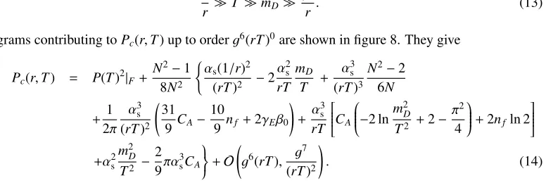
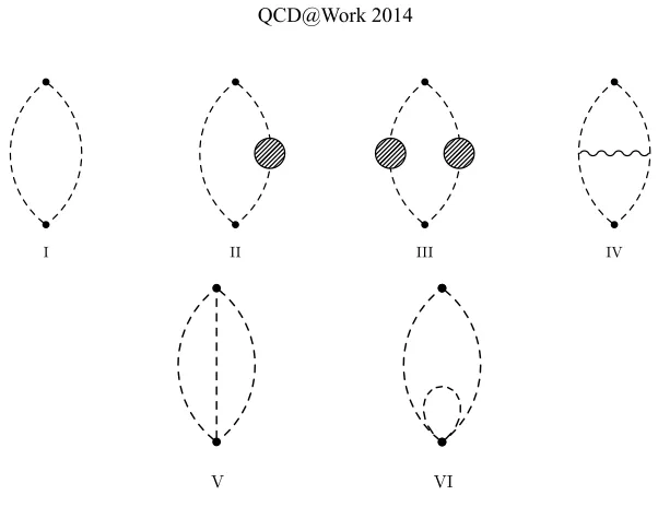
Divergences appear when all vertices are contracted to an intersection point. We restrict here to intersection divergences of a cyclic Wilson loop. In this case, when one vertex is on the string, if every vertex can be contracted to the intersection, then the contribution of the diagram cancels because of cyclicity (see [5]). Moreover, if all vertices are on a quark line, then the diagram contributes equally to the Polyakov loop, which is finite after charge renormalization. Hence a connected diagram cannot give rise to an intersection divergence, because either we are in one of the situations above, or it has at least one uncontracted vertex and therefore it is finite. Examples of intersection divergent diagrams in a cyclic Wilson loop are the last two diagrams shown in figure 5.
1.4 Renormalization
Figure 5. Some diagrams contributing toWc(r,T). Diagrams in the top row are connected and do not give intersection divergences. Diagrams in the second row: the first diagram has line vertices only on one quark line, so it also contributes to the Polyakov loop, which is finite after charge renormalization; the second diagram has vertices on a string and on one quark line and thus cancels through cyclicity; the third and fourth diagrams are divergent, because, due to the periodic boundary conditions, we can contract the line vertices of the respective one-gluon and three-gluon subdiagrams to an intersection point.
points connected by at most two Wilson lines to other intersection points (anglesθk) and with cusps
(anglesϕl) gets renormalized as
Wi(R)
1i2...ir =Zi1j1(θ1)Zi2j2(θ2)· · ·Zirjr(θr)Z(ϕ1)Z(ϕ2)· · ·Z(ϕs)Wj1j2...jr, (7)
where the indicesikand jklabel the different possible path-ordering prescriptions at the intersection
points, the coupling inWi(R)
1i2...ir is the renormalized coupling and the matricesZ are renormalization
matrices. The loop functions are color-traced and normalized by the number of colours, which ensures that all loop functions are gauge invariant. For some additional remarks on the applicability of the renormalization formula (7) we refer to [7].
2 Polyakov loop
We consider here the Polyakov loop average defined in (1). It is convenient to compute it in the static gauge,∂0A0(x)=0, so that:
L(x)=exp igA0
(x) T
. (8)
Propagators may be split into a static and a non-static component:
D00(ωn,k) =
=δn0 k2,
Di j(ωn 0,k) =
=1 ω2
n+k2
δi j+
kikj
ω2
n
(1−δn0),
Di j(ωn =0,k) =
=1 k2
δi j−(1−ξ)
kikj
k2
δn0,
Dghost(ωn,k) =
=Up to g4 the diagrams contributing to P(T)|
R in the static gauge are shown in figure 6. They
give [9]:
P(T)|R=1+
CRαs 2
mD
T +
CRα2s 2
⎡ ⎢⎢⎢⎢⎣CA
⎛ ⎜⎜⎜⎜⎝lnm
2
D
T2 + 1 2 ⎞
⎟⎟⎟⎟⎠−nfln 2
⎤
⎥⎥⎥⎥⎦+O(g5), (9) whereCR is the Casimir of the color representation R: CF = (N2−1)/(2N),CA = N. The
loga-rithm, lnm2
D/T2, signals that an infrared divergence at the scaleT has canceled against an ultraviolet
divergence at the scalemD.
+ + +. . .
Figure 6.Diagrams contributing toP(T)|Rup tog4in the static gauge.
In [9], also some higher order terms have been calculated. In particular, non-static modes at the scalemDcontribute with
δP(T)NS,mD =
3g4C
R
4(4π)3 mD
T
β0ln μ
4πT 2
+2β0γE+
11 3 CA−
2
3nf(4 ln 2−1)
, (10)
whereβ0is the coefficient of the one-loop beta function. This contribution fixes the renormalization scale ofg3in (9) toμ∼4πT. Furthermore, the diagram shown in figure 7 provides the leading con-tribution to theCasimir scalingviolation of the Polyakov loop average (i.e. the leading contribution whose color structure is not linear inCR):
δP(T)Casimir viol.=
3C2R−CRCA 2 α2 s 24 m D T 2 . (11)
As we remarked above, this contribution, which involves only static loops, comes from integrating over momenta scaling likemD.
2.1 Comparison with the literature
In 1981, Gava and Jengo obtained in the pure gauge case (nf =0) [10]:
P(T)GJ=1+ CRαs
2 mD
T +
CRCAα2s 2
⎛ ⎜⎜⎜⎜⎝lnm
2
D
T2 −2 ln 2+ 3 2 ⎞
Figure 7. Leading diagram contributing to the Casimir scaling violation of the Polyakov loop average in the static gauge.
This result disagrees with (9). The origin of the disagreement can be traced back to a missed resum-mation of the Debye mass in the temporal gluons contributing to the static gluon self energy.
Equation (9) agrees instead with the determination of Burnier, Laine and Vepsäläinen, who use a dimensionally reduced effective field theory framework in a covariant or Coulomb gauge [11].
3 Polyakov loop correlator
In [9], the Polyakov loop correlator (3) has been evaluated, assuming the following hierarchy of scales:
1
r T mD
g2
r. (13)
Diagrams contributing toPc(r,T) up to orderg6(rT)0are shown in figure 8. They give
Pc(r,T) = P(T)2|F+
N2−1 8N2
α s(1/r)2 (rT)2 −2
α2 s rT
mD
T +
α3 s (rT)3
N2−2 6N
+2π1 α3s (rT)2
31
9CA− 10
9 nf+2γEβ0
+α3s rT ⎡ ⎢⎢⎢⎢⎣CA
⎛ ⎜⎜⎜⎜⎝−2 lnm
2
D
T2 +2− π2
4 ⎞
⎟⎟⎟⎟⎠+2nfln 2
⎤ ⎥⎥⎥⎥⎦
+α2 s
m2
D
T2 − 2 9πα
3
sCA⎫⎪⎬⎪⎭+O
g6(rT), g7 (rT)2
. (14)
3.1 Comparison with the literature
In 1986, Nadkarni calculated the Polyakov loop correlator assuming the hierarchy T 1/r ∼ mD[12]. Whenever the previous results do not involve the hierarchyrT 1, they agree with
Nad-karni’s ones expanded formDr1.
Effective field theory approaches for the calculation of the correlator of Polyakov loops for the sit-uationsmD>∼1/r[13] andT 1/r[12] have been developed since long. In those situations, the scale
1/rwas not integrated out, and the Polyakov-loop correlator was described in terms of dimensionally reduced effective field theories of QCD, while the complexity of the bound-state dynamics remained implicit in the correlator. Those descriptions are valid for largely separated Polyakov loops when the correlator is either screened by the Debye mass, formDr∼1, or the mass of the lowest-lying glueball,
V VI
Figure 8.Diagrams contributing toPc(r,T) up to orderg6(rT)0in the static gauge.
The Polyakov loop correlator can be put in the form
Pc(r,T)=
1 N2
e−fs(r,T,mD)/T+(N2−1)e−fo(r,T,mD)/T+Oα3
s(rT)4 , (15)
wherefscan be identified with theQQ color-singlet free energy¯ and fowith theQQ color-octet free¯
energy. The color-singlet quark-antiquark potential has been calculated in real-time formalism in the same thermodynamical situation considered here in [14]. The comparison of fs with the real-time
potential leads to the conclusion that the two cannot be identified since the real part of the real-time
potential differs from fs(r,T,mD) by
1 9πNCFα
2 srT2−
π 36N
2C
Fα3sT. Moreover, the real-time potential has also an imaginary part that is absent in the free energy.
Jahn and Philipsen have analyzed the gauge structure of the allowed intermediate states in the correlator of Polyakov loops [15]: the quark-antiquark component, ϕ, of an intermediate state made of a quark located in x1 and an antiquark located in x2 should transform as ϕ(x1,x2) → Ω(x1)ϕ(x1,x2)Ω†(x2) under a gauge transformationΩ. The decomposition of the Polyakov loop cor-relator in terms of a color singlet and a color octet corcor-relator is in accordance with that result, for both aQQ¯singlet and octet field transform in that way. We remark, however, a difference in language: sin-glet and octet in fsand forefer to the gauge transformation properties of the quark-antiquark fields,
while, in [15], they refer to the gauge transformation properties of the physical states. In that last sense octet states cannot exist as intermediate states in the correlator of Polyakov loops.
4 Cyclic Wilson loop
Differently fromP(T) andPc(r,T), the cyclic Wilson loop,Wc(r,T), defined in (4), is divergent after
needs to care only about the two endpoints, for the Wilson loop contour does not lead to divergences in the other ones. As a special case of (7), a cyclic Wilson loop renormalizes as [5]:
Wc(R)
Pc
=
Z 1−Z
0 1 Wc Pc , (16) where
Z =1+Z1αsμ−2ε+Z2
αsμ−2ε 2
+O(α3
s). (17)
The renormalization constantZ1is given by
Z1=− CA
π 1
ε. (18)
The renormalization constantZ2reabsorbs all divergences of the typeα3s/(rT) showing up in the cyclic Wilson loop, whereas, all other divergences atO(α3s) are reabsorbed byZ1(combined withPc(r,T) at
O(α2
s), see (14))!
The renormalization group equations read ⎧⎪⎪⎪ ⎪⎪⎨ ⎪⎪⎪⎪⎪ ⎩ μ d dμ W(R)
c −Pc
=γW(R)
c −Pc
μd dμαs=−
α2 s
2πβ0+O(α3s)
, (19)
whereγis the anomalous dimension ofWc(R)−Pc:
γ≡ 1 Zμ
d
dμZ=2CA
αs
π +O(α2s). (20)
The solution of the renormalization group equations at one-loop is
Wc(R)−Pc
(μ)=Wc(R)−Pc
(1/r)
α s(μ) αs(1/r)
−4CA/β0
. (21)
In the MS-scheme, up to order g4 and including all termsα
s/(rT)×(αslnμr)n, assuming the hierarchy of scales 1/rT mDg2/r, the final expression for the cyclic Wilson loop reads [5]
lnWc(R)(r,T;μ) =
CFαs(1/r) rT
1+4παs
31
9CA− 10
9 nf
+2β0γE
+αsCA
π ⎡ ⎢⎢⎢⎢⎢
⎣1+2γE−2 ln 2+
∞ !
n=1
2(−1)nζ(2n)
n(4n2−1) (rT) 2n
⎤ ⎥⎥⎥⎥⎥ ⎦⎫⎪⎪⎬⎪⎪⎭
+4παsCF
T
d3k (2π)3
eir·k−1 ⎡ ⎢⎢⎢⎢⎢
⎣k2+ Π1(T) 00(0,k)
−k12 ⎤ ⎥⎥⎥⎥⎥
⎦+CFCAα2s
+CFαs rT ⎡ ⎢⎢⎢⎢⎢ ⎣ α s(μ) αs(1/r)
−4CA/β0 −1
⎤ ⎥⎥⎥⎥⎥
⎦+Og5, (22)
whereΠ(00T)(0,k) is the (known) thermal part of the gluon self-energy in Coulomb gauge.
the same renormalization equation (16) with the same renormalization constantZcomputed at short distances.
Finally, we observe that loop functions have, in general, power divergences, which factorize and exponentiate to give a factor exp [ΛL(C)], whereL(C) is the length of the contourCandΛis some linearly divergent constant. Only in dimensional regularization such linear divergences are absent, but they would be present in other schemes such as e.g. lattice regularization [8]. An efficient way to calculate the exponent of Wilson loops is the so-called replica trick [16, 17]. This consists in calculating the exponent of a Wilson loopW, i.e. lnW, by computing the left-hand side of
W1·W2· · ·WN=1+NlnW+O(N2), (24)
whereWiis theith copy ofW in a replicated theory of QCD not interacting with the others. A
renor-malized combination is then [7]
exp"−2ΛF/T −ΛAr# ×Z ×$Wc(r,T)−Pc(r,T)%, (25)
whereZis now understood in the same renormalization scheme as the linear divergences.
4.1 Implications for lattice QCD
The renormalization ofWcallows a proper calculation of this quantity on the lattice. The right quantity
to compute is the multiplicatively renormalizable combinationWc−Pc(see (25)). A finite quantity is
(Wc−Pc)(r,T)
(Wc−Pc)(r0,T)×
(Wc−Pc)(2r0−r,T) (Wc−Pc)(r0,T)
, (26)
wherer0is a given distance.
Acknowledgements
I acknowledge financial support from the DFG cluster of excellence “Origin and structure of the universe” (http://www.universe-cluster.de).
References
[1] L. D. McLerran and B. Svetitsky, Phys. Rev. D24, 450 (1981).
[2] N. Brambillaet al., CERN-2005-005, (CERN, Geneva, 2005) [arXiv:hep-ph/0412158]. [3] V. S. Dotsenko and S. N. Vergeles, Nucl. Phys. B169, 527 (1980).
[4] G. P. Korchemsky and A. V. Radyushkin, Nucl. Phys. B283, 342 (1987).
[6] R. A. Brandt, F. Neri and M. a. Sato, Phys. Rev. D24, 879 (1981).
[7] M. Berwein, N. Brambilla and A. Vairo, Phys. Part. Nucl. 45, no. 4, 656 (2014) [arXiv:1312.6651 [hep-th]].
[8] A. M. Polyakov, Nucl. Phys. B164, 171 (1980).
[9] N. Brambilla, J. Ghiglieri, P. Petreczky and A. Vairo, Phys. Rev. D 82, 074019 (2010) [arXiv:1007.5172 [hep-ph]].
[10] E. Gava and R. Jengo, Phys. Lett. B105, 285 (1981).
[11] Y. Burnier, M. Laine and M. Vepsäläinen, JHEP1001, 054 (2010) [Erratum-ibid.1301, 180 (2013)] [arXiv:0911.3480 [hep-ph]].
[12] S. Nadkarni, Phys. Rev. D33, 3738 (1986).
[13] E. Braaten and A. Nieto, Phys. Rev. Lett.74, 3530 (1995) [hep-ph/9410218].
[14] N. Brambilla, J. Ghiglieri, A. Vairo and P. Petreczky, Phys. Rev. D 78, 014017 (2008) [arXiv:0804.0993 [hep-ph]].
[15] O. Jahn and O. Philipsen, Phys. Rev. D70, 074504 (2004) [hep-lat/0407042].
[16] E. Gardi, E. Laenen, G. Stavenga and C. D. White, JHEP1011, 155 (2010) [arXiv:1008.0098 [hep-ph]].