Different approaches to TMD Evolution with scale
John Collins1,a
1104 Davey Lab, Penn State University, University Park PA 16802, USA
Abstract.Many apparently contradictory approaches to TMD factorization and its non-perturbative content exist. This talk evaluated the different methods and proposed tools for resolving the contradictions and experi-mentally adjudicating the results.
1 Introduction
In the literature there is a bewildering variety of methods for using transverse-momentum-dependent (TMD) par-ton densities and the associated factorization properties of cross sections. Taken at face value, many of the methods and their uses appear incompatible or contradic-tory, especially as regards the non-perturbative contribu-tions. The problems are particularly important when plan-ning new experiments to measure polarization-dependent TMD quantities like the Sivers function, since the non-perturbative part of TMD evolution can notably dilute them as energy is increased.
In this talk, I examined and evaluated some of the different methods. I proposed a systematic approach to test treatments of the non-perturbative contributions from large transverse distances (bT), both from theoretical and phenomenological view points. Then I proposed system-atic modifications to the standard parameterizations of the large-bT behavior that could resolve contradictions, espe-cially as regards the apparently incompatible phenomenol-ogy of the function controlling evolution of TMD densi-ties. The methods will pinpoint the experimental condi-tions needed to give incisive experimental probes of the contradictory theoretical statements.
2 The need for and existence of non-trivial
QCD contributions to TMD cross
sections
In this article, I use the Drell-Yan process to illustrate is-sues that apply to TMD factorization in general.
For the transverse-momentum distribution in the Drell-Yan process, the simplest model is the parton model, where the TMD cross section is a convolution of the TMD densities for the annihilating quark and antiquark, and the TMD densities do not evolve. In the parton model, the transverse momentum of the Drell-Yan pair directly probes the intrinsic transverse momentum distribution of the quark and antiquark inside their parent hadrons.
ae-mail: [email protected]
2.1 Experimental view
That the parton model description is inadequate in reality (and hence in QCD) is shown by the data in Fig. 1. The graphs also contain several QCD fits to the data. In plot (a) is shownEdσ/d3qfrom the E605 experiment at relatively low Q = 7–18 GeV and √s = 38.8 GeV. The width is around 1 GeV.
In plot (b) is shown dσ/dqTfrom the CDF experiment for Z production at √s = 1800 GeV. This has a much larger width, around 3 GeV. This value is much larger than for the lower energy data, and it also appears incompatible with any reasonable distribution of purely intrinsic trans-verse momentum. It indicates substantial evolution effects, a specific effect of QCD and other gauge theories.
There is an apparent dramatic difference between the plots atqT=0. This is merely an artifact of the normaliza-tion of the plotted cross secnormaliza-tion: Plot (b) has an extra factor ofqT, which gives a kinematic zero at the origin; for this plot a sensible measure of the width of the distribution is the position of the peak.
The values of parton xare characterized by the ratio Q/√s, which is quite different for the two plots. So inter-preting the difference between the widths as being associ-ated with evolution with respect toQis not totally unam-biguous; this is recurrent problem. Actual fits [1, 2] use other data as well, and appear to unambiguously manifest that there isQdependence at fixedx.
2.2 Need for evolution from QCD
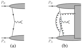
That QCD requires substantial modifications to the parton model is shown on the theoretical side by examining typi-cal graphs that contribute. In Fig. 2(a) is shown the graph-ical structure of the amplitude for the Drell-Yan process in the parton model. One quark or antiquark out of each of the high-energy incoming hadrons annihilates to make the Drell-Yan pair; the remaining “spectator” parts of the hadrons continue into the final state unchanged, with a big rapidity gap between them. In the parton model, other con-tributions are assumed to be power suppressed.
C
Owned by the authors, published by EDP Sciences, 2015
(a)
0.01 0.1 1
0 0.2 0.4 0.6 0.8 1 1.2 1.4
E605 Data
Data
Normalized LY-G Fit
Normalized DWS-G Fit Normalized BLNY Fit
q T (GeV)
E
d dq
y
3
3
00
3
σ
pb
GeV
nucleon
at
-2
⎛ ⎝⎜ ⎞ ⎠⎟
=
.
(b)
0 1 0 0 2 0 0 3 0 0 4 0 0 5 0 0 6 0 0 7 0 0 8 0 0
0 5 1 0 1 5 2 0
CDF Z Run 1
Data
Normalized LY-G Fit
Normalized DWS-G Fit Normalized BLNY Fit
q T (GeV) d dq
T
σ
pb
GeV
⎛ ⎝ ⎞ ⎠
Figure 1. The transverse-momentum distribution in the Drell-Yan process at different values ofQand √s, showing data from the E605 and CDF experiments, together with some fits to the data using TMD factorization. (Adapted from plots by Landry et al. [1].)
PB
PA
PB
PA
(a) (b)
Figure 2. For the Drell-Yan process: (a) Parton model graphs; (b) Examples of leading QCD graphs.
However, in QCD there are many other contributions that are not suppressed, as in the example in Fig. 2(b). First, there are final-state interactions that must exist to neutralize the color of the spectator parts. Also, many fur-ther contributions exist: Gluons of any rapidity within the kinematic range set by the incoming hadrons can connect any of the other lines, including all of: the active quarks,
Fourier trans. of p|ψ¯WLψ|p
Figure 3. Examples of graphs for parton density with Wilson line.
the spectator parts, and the final-state interaction compo-nent. Individual graphs do not give a factorized structure. But at leading power inQ, Ward identities and other meth-ods can be used to convert the sum over graphs to a fac-torized form. The Ward identities are somewhat unusual, and details can be found in [3, Sec. 11.9]. (Earlier lit-erature is lacking fully explicit formulations and proofs.) One consequence is that the parton densities must be de-fined with Wilson lines, as in Fig. 3. Effectively the Ward identities convert misattached gluons, that link regions of the graph with opposite rapidities, to attachments to Wil-son line operators. Further complications involve potential double counting of contributions from different kinematic regions of internal momenta, which must be suitably com-pensated, and the presence of a soft factor that in recent formulations is absorbed into a redefinition of the TMD densities.
The actual definition of the parton densities is such that the parton densities have extra scale arguments, and must evolve with energy. QCD thereby substantially violates the prediction of the pure parton model that the shape of transverse-momentum distribution scales with energy. The broadening arises because gluons are emitted roughly uni-formly into the available range of rapidity, which increases with energy. This applies to both perturbative and non-perturbative gluons.
3 TMD factorization (modernized
Collins-Soper form)
In this section I summarize the formulae of TMD factor-ization in the form I gave in [3]; detailed proofs were given there. Then then I remark on the location of the non-perturbative information.
3.1 TMD factorization
The factorization formula itself for the Drell-Yan cross section is
dσ d4qdΩ =
2 s
j
d ˆσj¯j(Q, μ)
dΩ ×
×
eiqT·bTf˜
j/A(xA,bT;ζA, μ) ˜fj/¯B(xB,bT;ζB, μ) d2bT
+poln. terms+high-qTterm+power-suppressed. (1)
Here, d ˆσ is the hard scattering coefficient, while the ˜
The evolution equations are
∂ln ˜ff/H(x,bT;ζ;μ)
∂ln√ζ =
˜
K(bT;μ), (2)
d ˜K
d lnμ=−γK(αs(μ)), (3)
d ln ˜ff/H(x,bT;ζ;μ)
d lnμ =γf(αs(μ); 1)− 1
2γK(αs(μ)) ln ζ μ2.
(4) Here, ˜K(bT;μ) is a defined function that controls the evolu-tion of the TMD pdfs and fragmentaevolu-tion funcevolu-tions of light quarks with respect to theζparameter.
In the parton model, the integral over all transverse momentum of a TMD parton density is the corresponding integrated, or collinear parton density. Equivalently, when the TMD densities are transformed to transverse coordi-nate space, the integrated density equals the TMD density at zero transverse separation. In any renormalizable quan-tum field theory, this result generally needs to be modi-fied. Instead, there is a kind of operator-product expansion (OPE) that expresses the TMD density at smallbTin terms of the integrated densities:
˜
ff/H(x,bT;ζ;μ)=
j
1+
x− ˜
Cf/j(x/xˆ,bT;ζ, μ, αs(μ))×
×fj/H( ˆx;μ) d ˆx
ˆ x + O
(mbT)p. (5)
The coefficients are perturbatively calculable provided that the TMD densities are evolved to scales that avoid large logarithms. The lowest-order value of the coefficients is δj fδ(x/xˆ−1), which is the parton model result.
3.2 Location of non-perturbative information
The TMD-specific non-perturbative information is at large-bT. Given the existence of the evolution equations, the necessary information is
• In the parton densities at large bT f˜j/A(xA,bT;ζA, μ) at one particular scale. One may choose to label this the “intrinsic transverse momentum” distribution if the scale is low, although this terminology is not entirely accurate.
• In the evolution kernel ˜K(bT;μ) at largebT. This gives a universal character to the evolution, and can be charac-terized as giving the effect of “soft glue per unit rapid-ity”.
Predictions for cross sections can only be made with the aid of phenomenological fits for these functions, and/or with the aid of non-perturbative theoretical modeling and calculation. The predictive power of the formalism stems from the universality of these functions: they can be mea-sured from a limited set of data and used to predict cross sections in many other situations, with the aid of evolution and of perturbative calculations of the remaining quanti-ties needed.
The OPE at small-bTalso needs the values of the ordi-nary integrated parton densities. These are obtained from fits to other data than is relevant for TMD factorization. This part of the non-perturbative information is therefore the same as in collinear factorization.
4 Formalisms used
A list of some of the formalisms that have been used in recent years is:
Parton model:Here QCD complications, especially TMD evolution, are ignored.
Non-TMD formalisms:These eschew the use of TMD densities in favor of collinear factorization and a resum-mation of large logarithms in the massless hard scattering. An old example is by Altarelli et al. [4]; a recent one is by Bozzi et al. [5].
Original CSS:Here a non-light-like axial gauge was used to define TMD densities without Wilson lines, and a soft factor appeared in the TMD factorization formula.
Ji–Ma–Yuan [6]:They implemented the CSS method with gauge-invariant TMD densities with non-light-like Wilson lines. They still had a soft factor, and used another parameterρbeyond the scale parameters of CSS.
New CSS:Here [3] there is a clean up relative to the orig-inal CSS version, Wilson lines are mostly light-like, and (square roots of) the soft factor are absorbed into TMD densities, in such a way that rapidity divergences associ-ated with light-like Wilson lines cancel.
Becher–Neubert (BN) [7]:This work uses SCET. TMD parton densities appear, but they are never finite.
Echevarría–Idilbi–Scimemi [8]:This is a SCET-based formalism, but with a different regulator to handle the di-vergences given by light-like Wilson lines than is used in the CSS and BN formalisms.
Mantry–Petriello [9, 10]:Another SCET-based method.
Boer [11], Sun-Yuan [12, 13]:These authors start from the CSS formalism, but make certain approximations. Sun and Yuan use no non-perturbative function for TMD evo-lution.
There is disagreement on size of non-perturbative con-tribution to evolution, i.e., on the form at largebT of the function that CSS call ˜K(bT); there is even disagreement as to whether this non-perturbative contribution exists.
5 Examination of some of the methods
5.1 Parton Model
high-qTcorrection term is ignored. The parton-model ap-proximation is typically used to fit data at relatively low energies compared with the earlier Drell-Yan fits. At these energies, a particular interest is in fitting polarization-dependent functions like the Sivers and Collins functions, e.g., [14, 15]. Typically a Gaussian ansatz is used for the shape of the TMD functions, e.g., [14].
The OPE (5) for the TMD densities at smallbTshows that the Gaussian ansatz cannot be exactly correct and that the Gaussian ansatz will fail once large enough transverse momenta are considered. But it evidently allows a good fit to data at low energy.
The neglect of higher-order terms in the hard scattering is reasonable, sinceαs(Q) is small. It is also reasonable to neglect the high-qTcorrection whenqTis small enough compared withQ. However, in view of the TMD evolution effects definitely seen at highQ, omitting evolution is not correct when a broad enough range ofQis considered.
However, in reality it is found [16, 17] that the data indicates that between the energies of the HERMES and COMPASS experiments, TMD evolution appears to exist but is weak. A complication in coming to this conclusion is that in an experiment at fixed energy,xandQare highly correlated.
5.2 Methods without TMD functions
Some authors, e.g., Altarelli et al. [4] and Bozzi et al. [5], eschew completely the use of TMD densities. They use collinear factorization together with a resummation of large logarithms of Q/qT in higher orders of the mass-less hard scattering coefficient in the collinear factoriza-tion framework. If this were fully justified, it would im-prove predictive power, since the only non-perturbative in-formation used is in the ordinary integrated parton densi-ties.
However, the justification of collinear factorization uses approximations for largeQthat are valid only when qTis of order Qor whenqT integrated over. The logical foundation fails whenqTQ. The errors in collinear fac-torization relative to the true cross section are suppressed by powers not only ofΛ/Qbut also ofqT/Q. An impor-tant symptom of this is that in the leading power “twist-2” collinear factorization, the effects of Boer-Mulders and Sivers functions are missed, whereas at low transverse mo-mentum these functions given leading power effects. See Ref. [18] for a good description of this last issue.
Further, in the resummation formalism, integrals over scale include non-perturbative regions with, e.g.,αs(k2) at smallk. A proper TMD factorization shows what to in this region.
5.3 Original CSS
In the original CSS formalism [19, 20], TMD parton den-sities were defined in a non-gauge-invariant way with use of non-light-like axial gauge; this was used to cut offthe rapidity divergences that would appear if the most natu-ral definition, with light-cone gauge, were used. The CSS
evolution formula, of the form of (2), gave the dependence of TMD functions on this rapidity cut off. There was a separate soft function in the factorization formula. Fur-thermore the evolution equations have power-suppressed corrections, which are dropped in phenomenological ap-plications.
CSS recognized that there are non-perturbative effects at large transverse distance bT. To separate these from perturbatively calculable phenomena, they proposed [21] their b∗ prescription. The combination of TMD
factor-ization, TMD evolution and the definitions of the TMD densities etc determined what kinds of functions to use for parameterization of non-perturbative parts of the cross sec-tion.
Phenomenologically, classic fits to Drell-Yan with 5 GeV Q ≤ mZ were made by Landry et al. (BLNY) [1], and later by Konychev and Nadolsky (KN) [2].
On the theoretical side, a difficulty with the use of ax-ial gauge to define parton densities is that the singularities in gluon propagators prevent the direct use of the contour deformations that are used in showing that the effects of the Glauber region cancel in the inclusive Drell-Yan cross section. CSS did not present an explicit solution to this problem. Nevertheless the structure of the formula they presented for the solution of the evolution equations re-mains as an actually implemented method for comparison with data, and agrees with later results.
5.4 Ji-Ma-Yuan
Ji, Ma and Yuan [6] converted the CSS formalism so that the TMD densities were defined gauge-invariantly, with non-light-like Wilson lines. Their factorization formula still has a separate soft factor, like that of CSS. The way in which they derived factorization entail the use of an ex-tra (dimensionless)ρparameter in the hard scattering etc, withρbeing large. There are associated large logarithms, and theρparameter is in addition to the scale parameters of the CSS formalism. There should have been evolution equation forρ, but such an equation appears not to have been given.
I know of no fits that actually use this scheme. Fits continued to use the CSS method.
5.5 New CSS
In [3], I derived an updated, improved version of the CSS results. On the theoretical side:
• Covariant gauge was used throughout, with suitable Wilson lines in gauge-invariant definitions of all the TMD functions.
• Full proofs (at least to all orders of perturbation theory) were given, including a proof of cancellation of the ef-fects of the Glauber region that applies both to collinear and to TMD factorization. (This entails particular direc-tions for the Wilson lines.)
• As many Wilson lines were made light-like as possible. The limits are quite non-trivial to formulate, which is a problem that stymied Ji, Ma and Yuan.
• The evolution equations are strictly homogeneous. The result is substantially cleaner methods relative to the original CSS work. From a phenomenological viewpoint, the new results should be regarded as being at most a scheme change from the original CSS method, as repre-sented by the solution of the evolution equations.
5.6 Becher-Neubert
Becher and Neubert [7] obtained a kind of TMD factor-ization in the framework of soft-collinear effective theory (SCET) in the Beneke-Smirnov style. The results are in-tended to be valid for large QwithqT Q, but with a restriction toqT Λ(unlike the CSS framework, which does not have this last restriction). By the restriction to qT Λ, they evade issues of a full TMD formalism and the need for non-perturbative information at largebT. But this also means that their method does not apply in the re-gion of lowqT, which is of much experimental interest. Thus their methods also do not include the physics asso-ciated with Sivers and Boer-Mulders functions, etc, which at leading power show their characteristic effects primarily in the region of non-perturbativeqT.
Furthermore they could not define separate TMD pdfs; only the product of two TMD pdfs was defined and free of divergences. This represents an inadequacy of the Beneke-Smirnov approach.
However, the Becher-Neubert method has given an im-portant tool for NNLO calculations of the coefficient func-tions in the OPE (5) — see [22, 23].
5.7 Echevarría–Idilbi–Scimemi
Echevarría, Idilbi and Scimemi [8] also obtained TMD factorization in a SCET framework. Their methods are characterized by the use of strictly light-like Wilson lines, but with a different kind of regulator for the associated ra-pidity divergences. (I do not think it obeys gauge invari-ance, which causes considerable difficulty in constructing full proofs. Full proofs of factorization make essential use of Ward identities or some equivalent to combine and can-cel non-factorizing terms from individual graphs.)
As with the method of [3], they absorb soft factors into the definition of TMD parton densities, but in a simpler way that depends on their methodology. Individual TMD parton densities are defined, unlike the case for Becher and Neubert’s approach.
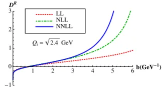
In phenomenological fits, Gaussian parameterizations are used for the TMD parton densities at an initial scale. But a claim is made that non-perturbative information is not needed in their equivalent of CSS’s ˜K function that controls the evolution of the shape of TMD functions. In-stead, for ˜K, they use a resummation of perturbation the-ory. This is applied up to a scale ofbT =4 GeV−1=0.8 fm or beyond.
In Fig. 4 is shown an example of their results for ˜K, in various approximations.
1 2 3 4 5 6bGeV 1
1 0 1 2 3D
R
NNLL NLL LL
Qi 2.4 GeV
Figure 4. Plot of DR(b
T;Qi) = −K˜(bT;Qi), from Melis, QCD Evolution 2014 workshop. Numerical results of three approximations are shown: leading logarithm (LL), next-to-leading-logarithm (NLL), and next-to-next-to-next-to-leading-logarithm (NNLL).
6 Geography of evolution of cross section
The evolution of TMD parton densities in formulated mul-tiplicatively in the space of transverse position. In Fig. 5 is plotted thebT-space integrand corresponding to the two cross section plots in Fig. 1. Up to an overall normaliza-tion factor, the integrand plotted isbT times the integrand in the TMD factorization formula (1) whenμ = Q. To get the cross section, this integrand is to be multiplied by the Bessel function J0(qTbT) and integrated overbT from zero to infinity. In general, in going from low to highQ, the peak region of the integrand migrates to ever-smaller values ofbT.
We now examine the plots with a black solid line and a purple dot-dashed line. These correspond to fits made to the same data by Konychev and Nadolsky [2] with the same theoretical conditions except that bmax = 1.5 GeV−1 = 0.3 fm andbmax =0.5 GeV−1 = 0.1 fm, re-spectively, for the two lines. At lower energies, in graph (a), the two plots do not differ greatly. At high energy, in graph (b), the two lines match even more closely up to aboutbT=0.8 GeV−1, and then they diverge strikingly, so that the line corresponding to the smaller value ofbmaxis a factor of about two below the other line at the right-hand edge of the graph. Although this is a large difference, it occurs in a region where the integrand is small, so that the large difference has little effect on the actual cross section. The calculation of the cross section is dominated by much smaller values ofbT, which are in a perturbative region.
In both cases, the non-perturbative part of ˜K(bT) was parameterized by a quadratic function ofbT, but the co-efficient is substantially larger for the fit with the small value ofbmax =0.5 GeV−1. The plot illustrates a general phenomenon. Although the integral to get the cross sec-tion needs an integral over allbT, up to∞, there is little sensitivity at large Qto the detailed properties of the in-tegrand at largebT, and hence little sensitivity to the non-perturbative dependence at largebT.
7 Standard fits of TMD evolution give bad
low-
Q
predictions
(a)
0.25 0.5 0.75 1 1.25 1.5 1.75 2
bGeV1 0
10 20 30 40
Nfit
1bW
b,Q,x
A
,xB
fb
GeV
pCu ΜΜX;s38.8 GeV; Q11 GeV; y0
bmax1.5 GeV1, C3b0, Nfit1.19 bmax1.5 GeV1, C32b0, Nfit1.05 bmax0.5 GeV1, C3b0, Nfit1.09 QiuZhang , bmax0.3 GeV1, Nfit1
(b)
Figure 5. Plots of thebT-space integrands corresponding to the
cross section plots in Fig. 1. Adapted from plots by Konychev and Nadolsky [2].
bT. When the TMD pdfs are evolved backwards, to lower Q, this results in unphysical behavior. To see this, consider the large-bTbehavior of the integrand for the cross section, as given in:
d2bTeiqT·bTe−b
2
T[coeff(x)+const.×ln(Q2/Q20)]. . . . (6)
Thex-dependent coefficient is to be obtained from a stan-dard Gaussian fit to data of TMD densities at some initial scale. The coefficient with the ln(Q2/Q2
0) factor in the ex-ponent results from applying the CSS equation (2) with a quadratic fit for ˜K(bT) at largebT.
At low enough Q, the coefficient of b2
T in the expo-nent reverses sign, so that the integral diverges at large bTinstead of converging. With the BLNY fit, this rever-sal of sign occurs [13] in a region where there is data and where it is reasonable to apply TMD factorization. This is illustrated in Fig. 6. Even with the KN fit using bmax=1.5 GeV−1, which gives a smaller coefficient ofb2
T in ˜K, the evolved exponent is well below what is needed to fit HERMES data.
2 5 10 20 50
0.1 0.0 0.1 0.2 0.3 0.4 0.5
Q GeV
Figure 6.Coefficient of−b2
Tin the exponent in Eq. (6), from Sun
and Yuan [13], as a function ofQatx=0.1. The blue dashed line is for the BLNY fit, and the red solid line for a KN fit with
bmax=1.5 GeV−1. The dot represents the value needed for SIDIS
at HERMES.
8 Systematic analysis of non-perturbative
part of evolution
I propose the following assertions as a starting point to resolve the apparent discrepancies and contradictions in the literature, concerning ˜K(bT) at largebT:
• This function (or something equivalent) is needed to im-plement correctly theQdependence of TMD cross sec-tions.
• SurelybT above about 3 GeV−1 = 0.6 fm is in domain of non-perturbative physics, since we know that the size of the proton is about 1 fm.
• It is difficult to avoid confounding x-dependence with Q-dependence of transverse-momentum distributions. In measuring ˜Kone must be careful to analyze data with differentQat the same value of partonx.
• Fig. 6 strongly suggests that evolution of the shape of TMD parton densities slows down at lowerQcompared with what happens in the data fit by BLNY and KN. • LowQinvolves larger (more non-perturbative)bTthan
highQ.
I propose the following general guidelines for modify-ing current parameterizations:
• One should assume that the KN form (with itsb2 Tform) is appropriate only for moderate bT, to fit the higher energy DY data correctly. KN is preferred here over BLNY both because it gives a better fit, and because its valuebmax=1.5 GeV−1=0.3 fm is not excessively con-servative.
• As can be seen from Fig. 5, the data used for the KN and BLNY fits constrain ˜K mostly at bT below about 2 GeV−1.
• But ˜K(bT) should flatten out at the higher values ofbT that are relevant for lowerQexperiments (HERMES and COMPASS, etc).
9
K
˜
at large
b
T9.1 Basic issues
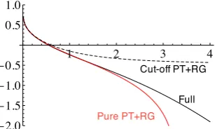
Figure 7. The components of ˜Kin (7). It is evaluated with the KN parameters forbmax =1.5 GeV−1=0.3 fm. The dashed line
is the cutoffversion ˜K(b∗, μ), calculated by perturbation theory and a standard renormalization-group (RG) improvement. The red solid line is the same thing but withbmax=∞, i.e., it is pure
RG-improved perturbation theory. It has a divergence at a finite valuebTbecause of the Landau pole in the coupling; perturbation
theory is evidently incorrect there. The solid black line gives the full KN result including the quadratic fittedgKfunction.
b∗prescription, one has
˜
K(bT, μ)=K(b˜ ∗, μ)−gK(bT;bmax), (7)
where
b∗= bT
1+b2 T/b2max
. (8)
In Eq. (7), ˜K(b∗, μ) is intended to be always perturbative,
and all non-perturbative behavior is parameterized in the functiongK. To illustrate this, Fig. 7 shows the decompo-sition of ˜Kwith the KN fit.
The fitted value of thegKfunction corrects the cut-off perturbative term, ˜K(b∗, μ), and brings the result for the
full ˜Kback to its RG-improved perturbative value forbT up to around bT = 2 GeV−1; only at higherbT does its curve move away from the diverging pure-PT line. One could therefore argue that the fitting has simply repro-duced perturbatively calculable behavior in this extended region, i.e., up to around bT = 2 GeV−1, perhaps also that the b∗ method could be improved, and perhaps that
bmax=1.5 GeV−1is still too conservative.
9.2 A possible parameterization
One naive idea is that instead ofb2
T, one uses the following parameterization forgK:
C b2
T+b21−bT−b1
. (9)
This goes to a constant asbT → ∞. There are two param-eters in (9). Better parameterizations can be found.
9.3 Simple ideas for physics constraints on large
bTbehavior
Given the evolution equation (2), one can characterize ˜
K(bT) as quantifying the effects of the emission of glue for each extra unit of available rapidity, when the energy of an experiment is increased, at fixedx.
So, for extra rapidity rangeΔy, let
• 1−cΔy=probability of no relevant emission • cΔy=probability of emitting particle(s)
• So another possibility for the non-perturbative part of ˜K is
˜
K(bT)NP=FT ofc −δ(2)(kT)+e−k
2
T/k
2
0 T/(πk2
0 T)
=c −1+e−b2Tk 2
0 T/4
. (10)
Here, I have made an ansatz that the transverse-momentum distribution of non-perturbative particle emission at low transverse momentum is Gaussian, motivated by com-monly used parameterizations.
We get yet another parameterization, now with quadratic behavior at small bT, and a non-infinite limit whenbT→ ∞.
Perhaps an exponential at largebT instead of a Gaus-sian would be better, given known general behavior of cor-relation functions at large Euclidean distances, as argued by Schweitzer, Strikman and Weiss [24].
10 Tool to compare different methods:
The
A
function
In a separate talk, I proposed a tool that can conveniently be used to quantitatively compare different methods for TMD factorization in a scheme-independent way. It will be described in much more detail in a forthcoming paper with Ted Rogers.
The motivation arises as follows:
• The shape change of transverse momentum distribution comes only frombT-dependence of ˜K in the CSS for-malism, or from some similar quantity.
• Generally in any TMD factorization scheme, the cross section can be written as a Fourier transformation:
dσ
d4q =normalization×
eiqT·bTW(bT ,s,x
A,xB) d2bT (11) • So let us define a scheme-independent function1
A(bT)=−∂ ∂ lnb2
T ∂
∂lnQ2ln ˜W(bT,Q,xA,xB)
CSS
= − ∂
∂lnb2 T
˜
K(bT, μ), (12)
where the second line gives its value in the CSS method. • QCD predicts that this function is:
– independent ofQ,xA,xB, – independent of light-quark flavor, – RG invariant,
– perturbatively calculable at smallbT, – non-perturbative at largebT.
It will be useful to compare the values of A(bT) that correspond to fits and formula in the different articles on the subject of TMD factorization and evolution. The val-ues of parameters where discrepancies occur can be used as a diagnostic: To show which experimental data will be most incisive in arbitrating the correctness of different treatments, and to diagnose which treatments are in dis-agreement with QCD and whether the disdis-agreements are significant.
11 Concluding remarks
• Surely we need non-perturbative contributions to TMD factorization. The values of bT that are important in the Gaussian parameterizations of TMD densities are in a region not far from the proton size. Every-body agrees that some parameterization of the non-perturbative properties of TMD densities is needed to describe data at low enough transverse momentum (and hence at largebT).
• Therefore one must also understand their evolution in this same non-perturbative region of largebT.
• According to established theorems, evolution of TMD functions is governed by a single universal function, ˜K or some equivalent.
• Extrapolation of earlier DY fits to use them at the values ofbTrelevant for lower energy SIDIS is incorrect. • It is essential to use better parameterizations of ˜K so
that at largebTits functional form flattens. The parame-terizations should be such that they retain compatibility with the evolution measured in Drell-Yan experiments, where substantially smaller values ofbT are important compared those needed for the data from the HERMES and COMPASS experiments.
• Physical and phenomenological arguments were given in support of these assertions.
• It is necessary to redo global fits with better parameteri-zations, and a clear sense of which data are relevant for which regions of transverse positionbT.
• In testing and measuring TMD evolution it is essential to ensure that the data being compared are at fixed xwith differentQ.
• A large coefficient for theb2
Tterm in ˜K(andgK) at large bT causes substantial dilution of the Sivers asymmetry, etc, at large Q, thereby requiring greater sensitivity in future higher-energy experiments. Getting improved un-derstanding and measurements of the non-perturbative part of TMD evolution is important to planning these future experiments.
Acknowledgments
This work was supported by the U.S. Department of En-ergy. I thank many colleagues for discussions, notably Ted Rogers and Ahmad Idilbi.
References
[1] F. Landry, R. Brock, P.M. Nadolsky, C.P. Yuan, Phys. Rev.D67, 073016 (2003),hep-ph/0212159 [2] A.V. Konychev, P.M. Nadolsky, Phys. Lett. B633,
710 (2006),hep-ph/0506225
[3] J.C. Collins, Foundations of Perturbative QCD (Cambridge University Press, Cambridge, 2011) [4] G. Altarelli, R.K. Ellis, M. Greco, G. Martinelli,
Nucl. Phys.B246, 12 (1984)
[5] G. Bozzi, S. Catani, D. de Florian, M. Grazzini, Nucl. Phys.B737, 73 (2006),hep-ph/0508068 [6] X.D. Ji, J.P. Ma, F. Yuan, Phys. Rev.D71, 034005
(2005),hep-ph/0404183
[7] T. Becher, M. Neubert, Eur. Phys. J. C71, 1665 (2011),1007.4005
[8] M.G. Echevarría, A. Idilbi, A. Schäfer, I. Scimemi, Eur. Phys. J.C73, 2636 (2013),1208.1281
[9] S. Mantry, F. Petriello, Phys. Rev. D81, 093007 (2010),0911.4135
[10] S. Mantry, F. Petriello, Phys. Rev. D84, 014030 (2011),1011.0757
[11] D. Boer, Nucl. Phys.B806, 23 (2009),0804.2408 [12] P. Sun, F. Yuan, Phys. Rev. D88, 034016 (2013),
1304.5037
[13] P. Sun, F. Yuan, Phys. Rev. D88, 114012 (2013),
1308.5003
[14] M. Anselmino, M. Boglione, U. D’Alesio, S. Melis, F. Murgia et al., Phys. Rev. D87, 094019 (2013),
1303.3822
[15] M. Anselmino, M. Boglione, U. D’Alesio, S. Melis, F. Murgia et al. (2011),1107.4446
[16] M. Anselmino, M. Boglione, S. Melis (2012),
1209.1541
[17] C. Aidala, B. Field, L. Gamberg, T. Rogers, Phys. Rev.D89, 094002 (2014),1401.2654
[18] A. Bacchetta, D. Boer, M. Diehl, P.J. Mulders, JHEP
08, 023 (2008),0803.0227
[19] J.C. Collins, D.E. Soper, Nucl. Phys. B193, 381 (1981), erratum:B213, 545 (1983)
[20] J.C. Collins, D.E. Soper, Nucl. Phys. B194, 445 (1982)
[21] J.C. Collins, D.E. Soper, G. Sterman, Nucl. Phys.
B250, 199 (1985)
[22] T. Gehrmann, T. Lubbert, L.L. Yang, Phys. Rev. Lett.
109, 242003 (2012),1209.0682
[23] T. Gehrmann, T. Luebbert, L.L. Yang, JHEP1406, 155 (2014),1403.6451
![Figure 6. Coefficient of −b2T in the exponent in Eq. (6), from Sunand Yuan [13], as a function of Q at x = 0.1](https://thumb-us.123doks.com/thumbv2/123dok_us/8184656.1366855/6.595.70.272.71.410/figure-coecient-t-exponent-eq-sunand-yuan-function.webp)