c
Owned by the authors, published by EDP Sciences, 2015
Neutron xyz – polarization analysis at a time-of-flight instrument
G. Ehlers1,a, J.R. Stewart2, P.P. Deen3and K.H. Andersen3
1Quantum Condensed Matter Division, Oak Ridge National Laboratory, Oak Ridge, TN 37831, USA 2ISIS, Rutherford Appleton Laboratory, Chilton, Didcot OX11 0QX, UK
3European Spallation Source ESS AB, Box 176, 22100 Lund, Sweden
Abstract. When implementing a dedicated polarization analysis setup at a neutron time-of-flight instrument with a large area detector, one faces enormous challenges. Nevertheless, significant progress has been made towards this goal over the last few years. This paper addresses systematic limitations of the traditional method that is used to make these measurements, and a possible strategy to overcome these limitations. This will be important, for diffraction as well as inelastic experiments, where the scattering occurs mostly out-of-plane.
1. Introduction
Direct geometry inelastic neutron time-of-flight (TOF) spectrometers are powerful instruments but they do not lend themselves very easily to performing polarization analysis [1–3]. These instruments feature very large detector arrays, covering up to∼30◦out of plane, which means that the scattered polarization must be analyzed over a large area. A second reason is that these instruments may use a wide range of wavelengths simultaneously, by employing the repetition rate multiplication (RRM) technique [4], which makes it difficult to optimize polarization analysis settings. Even so, significant progress has been made recently at various facilities [5–8].
Modern TOF instruments (elastic as well as inelastic) cover detector solid angles in excess of ∼2 sr, whereas existing instruments in which polarization analysis is a fixed installation have much smaller detectors. For example, one has∼0.4 sr at D7 [9,10],∼0.1 sr at DNS [11,12], and the WASP project at the Institut Laue-Langevin (ILL), which is currently under construction, is aiming for ∼0.2 sr [13]. These instruments use supermirror analyzers whereas the crystal analyzer instrument MACS at the National Institute for Standards and Technology (NIST) uses an array of wide angle3He analyzer cells [14]. The HYSPEC instrument at Oak Ridge National Laboratory (ORNL) is presently pursuing both options and will reach∼0.25 sr [15].
Magnetic neutron scattering has vector character, that is to say, the intensity and polarization of the scattered beam depend on the mutual direction of three vectors relative to each other: the scattering vector Q, the polarization direction of the neutron, and the direction of the magnetic moment from which the neutron is scattered. When one writes down expressions that connect the quantities one measures (x yz spin flip and non spin flip cross sections) and the quantities one is interested in (the nuclear coherent scattering N , nuclear spin-incoherent
ae-mail:[email protected]
scattering I , and magnetic scattering M), it turns out that some terms accidentally cancel if the scattering occurs in the x y plane (Q⊥z). As the use of the method can be
traced back to the 60s [16,17], this condition was always met, simply because neutron scattering instrumentation was nearly always confined to the x y plane. At a modern TOF instrument this is no longer true, and it is therefore worth going back to the basics of the technique and to develop the measurement protocol further, in particular to achieve a cleaner separation of M.
2. Scientific need for polarized neutrons
By far the greatest need for polarized neutrons is in magnetism. The direction in which research is currently developing emphasizes going towards increasingly com-plex materials, in which magnetic scattering features are often weak (due to spin-1/2 entities) or diffuse (because magnetic correlations are short-ranged) [18–21]. The widely adopted strategy to separate magnetic scattering (using unpolarized neutrons) with temperature variation (say, above and below a phase transition) cannot be applied with success if the magnitude of the magnetic scattering intensity is comparable – or weaker – than the variation with temperature of the nuclear scattering. In complex systems, it is more likely that lattice and spin dynamics overlap in (Q, ω) space, and may even
be “entangled” which is to say that an excitation may involve structural and magnetic degrees of freedom simultaneously [22]. Thus, in the future polarized neutrons will be increasingly indispensable for the separation of lattice and spin dynamics in magnetic systems, and also for independent measurements of transverse and longitudinal spin fluctuations.
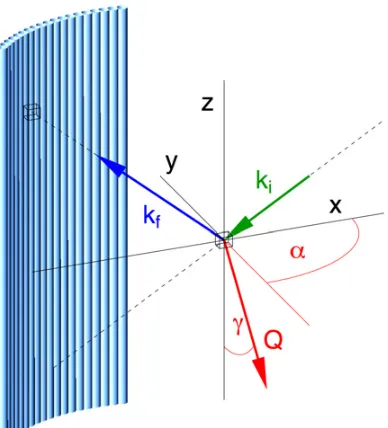
Figure 1. Sketch of the scattering geometry. The incident beam direction kiis in the scattering plane (the x y plane). The angleαis the angle between projection of the Qvector onto the scattering plane and the x direction. The angleγ is the angle between Q and the z axis.
of coherent and incoherent cross sections is thus readily available.
3. Polarization analysis with detector
coverage out of plane
The traditional way in which x yz−polarization analysis experiments are conducted involves preparing a linearly polarized neutron beam whose polarization is guided all the way through the instrument, up to the analyzing device which is situated behind the sample [2]. In the sample area the polarization direction is adiabatically rotated into different directions during the measurement. The setup also includes a flipping device which allows one to change the optical direction of the polarizer relative to the analyzer. One measures six cross sections (three polarization directions, spin flip and non spin flip for each). The directions are commonly referred to as the x, y and z directions, which are mutually perpendicular, and where
x and y make up the horizontal scattering plane and z is
vertical. The objective of such an experiment (elastic or inelastic) is to separate the nuclear coherent (N ), nuclear spin-incoherent (I ) and magnetic (M) contributions to the scattering. These three contributions manipulate the neutron spin during the scattering process in different ways, and keeping track of the polarization of the scattered beam enables their separation if the direction of the polarization is changed with respect to the scattering vector Q.
Figure1schematically shows the scattering geometry. Experimentally, the x yz coordinate system is set up by the devices that define the polarization directions. This does not necessarily line up with the ‘natural’ coordinate system of the host instrument, where one would choose one of the axes to be parallel to ki. The direction of the Q vector is
expressed with anglesαandγ(as shown in Fig.1) which, in general, one will have to calibrate (see below).
The “traditional” method, in which the polarization direction is adiabatically rotated in the x, y and z directions, is referred to here as the “6-pt method”. In such a measurement, the magnetic intensity M =M(Q, ω) can be separated by
M·1
2 ·
1−3 cos2γ= ∂2σ
∂ ∂ω
(x)
↓ + ∂2σ
∂ ∂ω
(y)
↓ −2· ∂2σ
∂ ∂ω
(z)
↓ =
2· ∂
2σ
∂ ∂ω
(z)
↑ − ∂2σ
∂ ∂ω
(x)
↑ − ∂2σ
∂ ∂ω
(y)
↑·
This was derived in previous work and is repeated here for convenience [2,3]. Note that M cannot be separated from cos2γ where γ is the out-of-plane angle according to Fig. 1. The cos2γ term vanishes in the horizontal
plane, where cos2γ =0. At an inelastic instrument, one
can determine cos2γ in each pixel and time bin from
the scattering triangle and feed it into this equation. At a diffraction instrument (no energy analysis) this is not possible and one measures in each pixel and time bin an averagecos2γweighed with the elastic vs. inelastic
scattering cross sections. However, even at an inelastic instrument one may find it preferable to be able to separate
M from cos2γ, for example, to reduce the impact of a deviation ofγ =0 from the exact vertical direction.
One can expand the 6-pt protocol by measuring a second set of polarization directions in the x y plane, which is rotated by 45◦ around the vertical axis [3]. This is referred to as the “10-pt method”, and the two new horizontal polarization directions are labelled “x +y” and
“x−y”. In this situation one can revise the above linear
combinations with coefficients that become dependent on the angleα, to cancel out the cos2γ terms. From “down” counts:
(2c0−4)·
∂2σ
∂ ∂ω
(x)
↓ +(2c0 +2)· ∂2σ
∂ ∂ω
(y)
↓
+(2−4c0)·
∂2σ
∂ ∂ω
(z)
↓ =−M·cos 2α (2c4−4)·
∂2σ
∂ ∂ω
(x+y)
↓ +(2c4 +2)· ∂2σ
∂ ∂ω
(x−y)
↓
+(2−4c4)·
∂2σ
∂ ∂ω
(z)
↓ =−M·sin 2α, and from “up” counts:
(2c0−4)·
∂2σ
∂ ∂ω
(x)
↑ +(2c0 +2)· ∂2σ
∂ ∂ω
(y)
↑
+(2−4c0)·
∂2σ
∂ ∂ω
(z)
(2c4−4)· ∂ 2σ
∂ ∂ω
(x+y)
↑ +(2c4+2)· ∂2σ
∂ ∂ω
(x−y)
↑
+(2−4c4)· ∂ 2σ
∂ ∂ω
(z)
↑ = +M·sin 2α,
where c0=cos2αand c4=cos2(α−π/4). One gets two
independent values for M, from “down” and “up” counts respectively, by writing
(M·cos 2α)·cos 2α+(M·sin 2α)·sin 2α=M.
The angle α can be determined in a self-consistent way during the instrument tuning procedure prior to the experiment. This tuning can be done using a standard sample with sufficiently strong paramagnetic intensity M (ideally MN,I ) by making use of the relations
tan 2α= ∂2σ
∂ ∂ω
(x+y)
↓ −
∂2σ
∂ ∂ω
(x−y)
↓ ∂2σ
∂ ∂ω
(x)
↓ − ∂2σ
∂ ∂ω
(y)
↓
= ∂2σ
∂ ∂ω
(x−y)
↑ −
∂2σ
∂ ∂ω
(x+y)
↑ ∂2σ
∂ ∂ω
(y)
↑ − ∂2σ
∂ ∂ω
(x)
↑ ·
For this purpose, the paramagnetic scattering must be
elastic and should be diffuse to give access to a wide Q
range. For example, spin ices and spin glasses do meet these criteria at low temperature [28,29].
The relative change of α between pixels and time bins can also be calculated from the instrument geometry without any ambiguity, becauseα is simply the in-plane angle of theQvector. For elastic scattering in the x y plane, αis linearly offset from half the scattering (polar) angleθ. Thus, the tuning only needs to compute an experimental offset which is the angle between the “x” direction and the incident beam. This makes it possible to construct a “map” of theαangle over the detector array quite accurately (at a diffraction instrument the scattering from the standard would have to be strictly elastic).
The new “10-pt” method was tested and verified in a show-case experiment that was reported earlier [3]. In the following, results from a more detailed Monte Carlo simulation are shown, which investigated in particular the consequences of quasielastic scattering.
4. Monte Carlo simulations
4.1. Detailed conditionsThe Monte Carlo simulation matched the D7 instru-ment [10] in most of the relevant parameters (distances, beam size and divergence, mean wavelength λ=4.8 ˚A, etc.). A pixilated two-dimensional detector was assumed that covered ±20◦ out of plane. In reality, the D7 detector array covers ±5◦ out of plane and the tubes are not position-sensitive. The simulation followed each neutron and its polarization through the instrument and
the scattering process, and recorded whether it would be counted in the spin flip or non spin flip channel. The simulated counts were then analyzed in exactly the same way as real data would be.
The virtual powder sample had Q independent nuclear spin incoherent (I ) and paramagnetic (M) scattering with a 1:10 intensity ratio. The nuclear coherent scattering (N ) was set to zero. Since the sum of the two contributions
M +I is a constant, any deviation in the magnetic from a
constant (in an analysis scheme that ignores cos2γ terms) will be reflected in the spin incoherent channel with inverse sign.
4.2. Monte Carlo results – elastic scattering
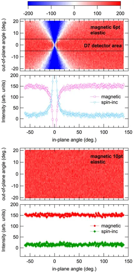
The top two panels in Fig.2 show the apparent magnetic scattering on a two-dimensional detector (top panel) with the traditional 6-pt setup, and the result of an analysis (second panel) that one would get with tubes that are not position sensitive (like at D7). Here one integrates the counts on the detector vertically and then applies the formalism to separate M. The angular range actually covered at D7 is also indicated in the figure. This comparison confirms that the corrections to the 6-pt method considered in this paper are relevant for D7 at low scattering angle.
In the forward direction one observes deviations from constant intensities below ∼20◦ scattering angle. This is a direct consequence of ignoring the cos2γ term
in the analysis. As expected, the effect becomes more pronounced as one goes away from the horizontal plane. This can be understood in simple terms at zero in-plane scattering angle, as there the scattering plane is vertical and the meanings of “x”, “y” and “z” are permuted. In this part of the detector, the linear combinations from the 6-pt equation would need to use different coefficients for the three directions. It can also be seen from the first equation given in Sect.3that M will change sign if cos2γ >1/3.
The bottom two panels in Fig.2show the true magnetic scattering on a 2D position sensitive detector with the new 10-pt setup. As expected, the input intensities were exactly recovered.
4.3. Monte Carlo results – quasielastic scattering
Figure 2. Top two panels: magnetic and spin incoherent scattering from the simulation, as analyzed with the 6-pt equation. Significant deviations from the input intensities are observed in the forward direction. The actual detector coverage at D7 is indicated. Bottom two panels: magnetic and spin incoherent scattering from the simulation, as analyzed with the 10-pt equations. Input intensities are exactly recovered.
On the other hand, the 10-pt method turns out to be quite sensitive to the scattering being quasielastic. The deviation of the scattering intensity in the forward direction is even more pronounced in this case.
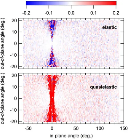
Figure 4 shows that the deviation of the scattering from the constant input intensity goes in parallel with a deviation of cos2αfrom the expected values. This figure shows the difference between cos2αvalues as determined
from the data (see Sect. 3) and from instrument tuning. While for elastic scattering (top panel in the figure) even in the forward direction the difference values scatter around zero, a strong net deviation is observed for the quasielastic case (bottom panel in the figure). This is not surprising: The data analysis in the lower part of Fig.3was performed
Figure 3. Top two panels: magnetic and spin incoherent scattering from the simulation, as analyzed with the 6-pt equations, in the presence of strong quasielastic scattering. Again, the actual detector coverage at D7 is indicated. Bottom two panels: magnetic and spin incoherent scattering from the simulation, as analyzed with the 10-pt equations, using the same dataset.
with an imposed map of theα angle that reflects strictly elastic scattering. If in fact the observed scattering is not elastic, within resolution, then one will get in each pixel a distribution of α and γ angles as Fig. 1 shows. The average truecos2αmust then deviate in each pixel from
the expected value. With the expected cos2αimposed,
the scattering intensity will naturally deviate from the input constant intensity. Thus the 10-pt method offers a manageable check whether the quasi-static approximation holds that one usually assumes in a diffraction experiment – one only has to compare experimental and expected cos2α and cos2γ values. This point was made by
Figure 4. Difference between cos2α as determined from the data and from instrument tuning for elastic scattering (top) and quasielastic scattering (bottom). In the forward direction one requires better counting statistics forcos2α. For elastic scattering the differences even out to zero whereas for quasielastic scattering a net positive difference is observed in the forward direction.
The value of the 10-pt protocol is that the angleαcan be determined modπ(as compared to modπ/2 with the 6-pt protocol) and that there is no information onγ whatsoever with the 6-pt method.
5. Conclusions
Adding a second x yz setup which is rotated by 45◦ around the vertical axis enables one to fully separate the three scattering contributions (N , I , M) from each other and from the scattering angles when considering scattering out of plane. At a diffraction instrument – without energy analysis – one generally relies on the quasi static approximation to hold and one will be sensitive to deviations from this approximation when studying a real material. In general, there will be hardly any signature of inelasticity in the measured diffraction intensities. However, in the angles cos2α and sin2γ as measured with diffraction such signatures will become apparent because inelasticity means that the direction of the Q
vector varies in one detector pixel and thus cos2α and
sin2γ will deviate from the values expected for elastic scattering. Therefore, 10-pt polarization analysis may provide valuable information on the inelasticity of the scattering even without energy analysis. This point was made by Sch¨arpf [2], and the idea was made use of by Murani et al. in-plane [30]. It is generalized in this paper to out-of-plane scattering.
At an inelastic instrument, strictly speaking, it is not necessary to employ the 10-pt method because the scattering triangle can be constructed in each pixel and time-of-flight bin without ambiguity (hence cos2α and
cos2γ are fully known everywhere). Still, it will be
beneficial to expand the traditional 6-pt protocol, because this allows one to fully cancel out the angles and minimize the set of assumptions in the data analysis. It may also be pointed out that at an instrument set up for the classical 6-pt scheme, the modified 10-pt scheme will be readily available, as one only rotates the horizontal field settings by 45◦to access the two additional polarization directions. The additional information is thus gained at near zero cost in terms of setup and measurement times.
G. E. acknowledges funding by the Scientific User Facilities Division, Office of Basic Energy Sciences, U. S. Department of Energy.
References
[1] M. B. Stone, J. L. Niedziela, D. L. Abernathy, L. DeBeer-Schmitt, G. Ehlers, O. Garlea, G. E. Granroth, M. Graves-Brook, A. I. Kolesnikov, A. Podlesnyak, and B. Winn, Rev. Sci. Instr. 85, 045413 (2014)
[2] O. Sch¨arpf and H. Capellmann, Phys. Stat. Sol. A 135, 359 (1993)
[3] G. Ehlers, J. R. Stewart, A. R. Wildes, P. P. Deen, and K. H. Andersen, Rev. Sci. Instr. 84, 093901 (2013)
[4] M. Russina and F. Mezei, Nucl. Instr. Methods in Phys. Res. A 604, 624 (2009)
[5] J. R. Stewart, K. H. Andersen, E. Babcock, C. D. Frost, A. Hiess, D. Jullien, J. A. Stride, J.-F. Barth´el´emy, F. Marchal, A. P. Murani, H. Mutka, and H. Schober, Physica B 385-386, 1142 (2006) [6] R. I. Bewley, J. W. Taylor, and S. M.
Benning-ton,Nucl. Instr. Methods in Phys. Res. A 637, 128 (2011)
[7] Q. Ye, T. R. Gentile, J. Anderson, C. Broholm, W. C. Chen, Z. DeLand, R. W. Erwin, C. B. Fu, J. Fuller, A. Kirchhoff, J. A. Rodriguez-Rivera, V. Thampy, T. G. Walker, and S. Watson, Physics Procedia 42, 206 (2013)
[8] T. Yokoo, K. Ohoyama, S. Itoh, J. Suzuki, M. Nanbu, N. Kaneko, K. Iwasa, T. J. Sato, H. Kimura, and M. Ohkawara, J. Phys.: Conf. Ser. 502, 012046 (2014)
[9] K. C. Rule, G. Ehlers, J. R. Stewart, A. L. Cornelius, P. P. Deen, Y. Qiu, C. R. Wiebe, J. A. Janik, H. D. Zhou, D. Antonio, B. W. Woytko, J. P. Ruff, H. A. Dabkowska, B. D. Gaulin, and J. S. Gardner, Phys. Rev. B 76, 212405 (2007)
[10] J. R. Stewart, P. P. Deen, K. H. Andersen, H. Schober, J.-F. Barth´el´emy, J. M. Hillier, A. P. Murani, T. Hayes, and B. Lindenau, J. Appl. Cryst. 42, 69 (2009) [11] W. Schweika and P. B¨oni, Physica B 297, 155 (2001) [12] W. Schweika, personal communication
[13] P. Fouquet, G. Ehlers, B. Farago, C. Pappas, and F. Mezei, J. Neutron Res. 15, 39 (2007)
Pike, G. Scharfstein, S. A. Smee, and R. Vilaseca, Meas. Sci. Technol. 19, 034023 (2008)
[15] C. Y. Jiang, X. Tong, D. R. Brown, H. Culbertson, M. K. Graves-Brook, M. E. Hagen, B. Kadron, W. T. Lee, J. L. Robertson, and B. Winn, Rev. Sci. Instr. 84, 065108 (2013)
[16] G. M. Drabkin, E. I. Zabidarov, Ya. A Kasman, and A. I. Okorokov, JETP Pisma 2, 541 (1965)
[17] S. V. Maleev, JETP Pisma 2, 545 (1965)
[18] M. A. de Vries, J. R. Stewart, P. P. Deen, J. O. Piatek, G. J. Nilsen, H. M. Rønnow, and A. Harrison, Phys. Rev. Lett. 103, 237201 (2009)
[19] G. J. Nilsen, F. C. Coomer, M. A. de Vries, J. R. Stewart, P. P. Deen, A. Harrison, and H. M. Rønnow, Phys. Rev. B 84, 172401 (2011)
[20] H. J. Silverstein, K. Fritsch, F. Flicker, A. M. Hallas, J. S. Gardner, Y. Qiu, G. Ehlers, A. T. Savici, Z. Yamani, K. A. Ross, B. D. Gaulin, M. J. P. Gingras, J. A. M. Paddison, K. Foyevtsova, R. Valenti, F. Hawthorne, C. R. Wiebe, and H. D. Zhou, Phys. Rev. B 89, 054433 (2014)
[21] K. Matan, Y. Nambu, Y. Zhao, T. J. Sato, Y. Fukumoto, T. Ono, H. Tanaka, C. Broholm, A. Podlesnyak, and G. Ehlers, Phys. Rev. B 89, 024414 (2014)
[22] L. P. Regnault, F. Tasset, J. E. Lorenzo, T. Roberts, G. Dhalenne, and A. Revcolevschi, Physica B 267-268, 227 (1999)
[23] B. J. Gabrys, Physica B 267-268, 122 (1999) [24] B. Farago, A. Arbe, J. Colmenero, R. Faust, U.
Buchenau, and D. Richter, Phys. Rev. E 65, 051803 (2002)
[25] A.-C. Genix, A. Arbe, S. Arrese-Igor, J. Colmenero, D. Richter, B. Frick, and P. P. Deen, J. Chem. Phys. 128, 184901 (2008)
[26] C. Pappas, G. Ehlers, and F. Mezei, Neutron
Scattering From Magnetic Materials (Elsevier,
Amsterdam, 2006) chapter 11, p. 521
[27] P. Schleger, G. Ehlers, A. Kollmar, B. Alefeld, J. F. Barthelemy, H. Casalta, B. Farago, P. Giraud, C. Hayes, C. Lartigue, F. Mezei, and D. Richter, Physica B 266, 49 (1999)
[28] G. Ehlers, A. L. Cornelius, T. Fennell, M. Koza, S. T. Bramwell, and J. S. Gardner, J. Phys.: Condens. Matter 16, S635 (2004)
[29] R. M. Pickup, R. Cywinski, C. Pappas, B. Farago, and P. Fouquet, Phys. Rev. Lett. 102, 097202 (2009)