The Green’s type matrices for consumption reduction
in a heterogeneous population model of TCLs with
diffusion
Md Musabbir Hossain1,∗ and Asatur Zh. Khurshudyan2,3
1 School of Mechatronic Engineering and Automation, Shanghai University, Shanghai 200444, China;
2 Institute of Natural Sciences, Shanghai Jiao Tong University, Shanghai, China;
3 Department on Dynamics of Deformable Systems and Coupled Fields, Institute of Mechanics, National
Academy of Sciences of Armenia; * Correspondence: [email protected];
Abstract: We consider a control problem for a diffusive PDE model of heterogeneous population of thermostatically controlled loads (TCLs) aiming to balance the aggregate power consumption within a given amount of time. Using the Green’s function approach, the problem is formulated as an approximate controllability problem for a residue depending on control parameters nonlinearly. A sufficient condition for approximate controllability is derived in terms of initial temperature distribution, operation time of TCLs and threshold value of the aggregate power consumption. Case studies allow to reveal the advantages of the proposed solution from numerical calculations point of view.
Keywords:PDE; Power Consumption; TCLs; Control; Minimization
1. Introduction
The usage of renewable energy sources is becoming more efficient as an alternative to power sources. Such advancement is exciting but performs significant challenges to the power industry. One of the main challenges is inherent variability in achieving significant penetration of renewable energy in modern power supply system [1]. Hence, a necessity of efficient power supply strategies, as well as balancing schemes in presence of intermittent power source occurs. One of best solutions is the elaboration of programmable calculating devices and power control means. Usually, thermostatically controlled loads (TCLs) are the typical control means in such systems and it may be a better option to provide necessary generation-balancing services. Because it is feasible for loads to compensate for power imbalances more rapidly than thermal generators [2]. By controlling aggregated TCLs, a promising opportunity can be obtained to mitigate the mismatch between power generation and demand, thus enabling renewable energy penetration and improving grid reliability [3].
TCLs account for more than one-third of electricity consumption in the United States [4]. Nowadays, the model of TCLs has gained extensive attention. Several methods have been used to model TCL populations. In [5], multi-agent reinforcement learning was developed for modeling of TCLs. Model accuracy scales linearly with the number of agents and gives evidence for the increased agency to further sensing, domain knowledge or data gathering time. In reference [6], multi-state operating reserve model of aggregate TCLs has been presented for power system short-term reliability evaluation. This analytical model for characterizing dynamics of the operating reserve is firstly developed based on the migration of TCLs’ room temperature inside temperature hysteresis band. A frequency control technique is used in the literature [7] based on decision tree concept by conducting TCLs at smart grids. A new controlling action is introduced here to limit the probabilities of separating loaded feeders from smart grids due to maloperation of under-frequency load shedding relays. In [8], authors propose a two-dimensional state-queuing modeling approach for the TCLs that increases the
state vector to a two-dimensional state matrix. This method improves the accuracy of the state-queuing model by adding temperature-varying-rate information.
Loads are usually regulated by switches between on and off regimes, as it is the case for example air conditioners. Switches are used when the thermostat temperature approaches the minimal or maximal admissible values. Thus, large populations of TCLs can be manipulated by small deviations of set-point temperature without causing any considerable inconvenience to consumers. In particular, a common temperature setpoint offset needs to be manipulated for controlling the aggregate power requirement of a population of TCLs [9]. This opportunity allows to develop efficient elaboration schemes aiming to reduce power consumption by a proper choice of the set-point temperature and the minimal and maximal admissible values of the temperature.
Currently, there exist multiple mathematical models allowing to describe the basic principle of TCL units. The simplest models are the hybrid ODE models that have been investigated in many previous works including [9–11]. In general statement, the hybrid ODE model provides a relationship for the conditioned mass temperature,Θias follows [11]:
˙
Θi= 1
RiCi
[Θ∞,i(t)−Θi(t)−Si(t)RiPi+w(t)], i=1, 2, . . . ,N, t>0, (1)
whereΘ∞,i(t)is the external temperature,Ci∈R+is the thermal capacitance (kWh/°C),Ri∈R+is the thermal resistance (°C/kW), andPi ∈ R(kW) is the cooling power supplied by the TCLs when switched on, the discrete functionSi∈ {0, 1}represents the hardwareon/off state, andwrepresents
unpredictable heat gains or losses due to occupancy: all the above quantities with a subscriptiare for theithload.
Except differential equation (1),Θiis subject to a natural constraint
Θmin,i≤Θi(t)≤Θmax,i, i=1, 2, . . . ,N, t>0. (2)
Here,Θmin,iandΘmax,iare the minimal and maximal admissible temperatures. Then, the set-point
temperature of theithload,Θsp,i, is determined in terms ofΘmin,iandΘmax,ias follows: Θsp,i =
Θmax,i+Θmin,i
2 .
On the other hand, introducing the width of the temperature band of theithload,σi, we have Θmin,i=Θsp,i−
σi
2, Θmax,i =Θsp,i+ σi
2. (3)
More sophisticated, but more realistic models are described by PDEs. Let the statesuandvdenote the density of TCL units per temperatureΘand timetin theonandoff states, respectively. Assume a homogeneous population of TCLs, i.e., assume that the parametersRi,Ci,Pi,Θmin,i, andΘmax,iare
equal for all TCLs omitting the subscriptifrom the corresponding symbols. Then, the couple(u,v) satisfies the following system of first order PDEs [3,12]:
[∂t−αλ(Θ,t)∂Θ−α]u(Θ,t) =0, [∂t+αµ(Θ,t)∂Θ−α]v(Θ,t) =0 (4) λ(Θmax,t)u(Θmax,t) =µ(Θmax,t)v(Θmax,t) (5) µ(Θmin,t)v(Θmin,t) =λ(Θmin,t)u(Θmin,t) (6) where
α= 1
RC >0, λ(Θ,t) =−(µ(Θ,t)−RP)>0, µ(Θ,t) =Θ∞(t)−Θ>0.
At this, some important characteristics as numbers of loads in theonandoffstates and aggregate power consumption are evaluated in terms of(u,v)as follows:
non(t) =
Z Θmax
Θmin
u(Θ,t)dΘ, no f f(t) =
Z Θmax
Θmin
v(Θ,t)dΘ,
κ(t) = P k
Z Θmax
Θmin
u(Θ,t) dΘ, (7)
wherekis the performance coefficient.
The quantitiesΘsp,iandσiare usually considered as control parameters in order to control the
aggregate power consumption (7). For a relevant study, see, e.g., [4].
2. A PDE model considering diffusion phenomenon
Numerical simulation of various TCL populations reveals a diffusive phenomenon. Therefore, in [3] a diffusion equation has been proposed for a proper analysis of heterogeneous population models. The model equations read as
Dλ[u] =0, Dµ[v] =0, t>0, Θ∈(Θmin,Θmax), (8) where
Dλ ≡∂t−β∂ΘΘ−αλ(Θ,t)∂Θ−α, Dµ≡∂t−β∂ΘΘ+αµ(Θ,t)∂Θ−α, andβis a diffusivity coefficient with unit (°C)3/s.
Homogeneous system (8) is equipped with the following boundary conditions:
λu−µv=0, Θ=Θmin,Θmax, t>0, (9) ∂Θu+∂Θv=0, Θ=Θmin,Θmax, t>0. (10) The following initial conditions are also given:
u(Θ, 0) =u0(Θ), v(Θ, 0) =v0(Θ). (11)
Remark 2. Note that system (8) is coupled via boundary conditions (9)–(10), ensuring that the total number of TCLs is conserved. Unlike the model without a diffusive term (see Remark1), analysis of (8)–(11) is sophisticated. 2.1. Solution via matrices of Green’s type
Let us derive the closed form solution of (8)–(11) by means of the concept of Green’s function. To this end, we introduce new functions
u(t) =θ(t−0)u(t), v(t) =θ(t−0)v(t),
whereθis the Heaviside function, andt−0 in its argument indicates that the pointt=0 is approached from the right. Then, (8) is reduced to
Following to [14], the general solution of (12)–(11) can be represented as follows:
u v
! =
Z t
0
Z Θmax
Θmin
G11 G12 G21 G22
!
u0(ϑ)δ(τ) v0(ϑ)δ(τ) !
dϑdτ=
= Z Θmax
Θmin
G11 G12 G21 G22
!
τ=0
u0(ϑ) v0(ϑ) !
dϑ,
(13)
whereGij = Gij(Θ,ϑ,t,τ),i,j = 1, 2, are the elements of the matrix of Green’s type. An efficient numerical scheme for computingGijhas been developed by Melnikov in [14].
Remark 3. Note that solution (13) is linear with respect to the initial state(u0,v0). 2.2. Aggregate power consumption
The closed-form solution (13) allows to express the aggregated power consumption in terms of system parameters. Substituting the firs raw of (13) into (7), we will obtain
κ(t) = P k
Z Θmax
Θmin Z Θmax
Θmin
[u0(ϑ)G11(Θ,ϑ,t, 0) +v0(ϑ)G12(Θ,ϑ,t, 0)]dϑdΘ. (14)
3. Control of the diffusive PDE model
In this section, we consider the problem of controlling the amount of the aggregate power consumption (7) by choosing the quantitiesΘspandσaccordingly. Such a problem for the simplest model described by (4) has been considered, e.g., in [?]. The problem is to choose appropriate values forΘspandσin order to ensure
R Θsp,σ= max
0≤t≤Tκ(t)−κ0≤ε, (15)
with a desired accuracyε>0. Here,κ0≥0 is a given threshold value of admissible consumption,T is the operation time of the TCLs. In other words, we chooseΘspandσin such a way that the total power consumption during the operation interval[0,T]does not exceed a desired amount.
Remark 4. Even though we callεan accuracy, it does not imply that it should be a small quantity. Indeed, as soon asκ0=0,εcan not be smaller than the minimal possible value ofκin[0,T]. On the other hand, when κ0>0, meaningful values ofε1.
Remark 5. Note that in the terminology of [13], this is an approximate controllability problem.
Since the mathematical model is linear in(u,v), for our purpose, we involve the Green’s function approach developed in [13]. Substituting (14) into (15), we make the dependenceR = R Θsp,σ explicit.
Remark 6. It should be noted thatRdepends onΘsp,σthrough the limits of integration, as well as through G11and G12. Thus, the minimization ofRis not that straightforward.
The main result of the paper can be stated in the following theorem.
Theorem 1. If for given u0, v0, T,κ0andε, there exist a bounded constant C Θsp,σ>0such that
uniformly for0≤t≤T,Θmin≤Θ,ϑ≤Θmax, then R Θsp,σ≤ P
kσ
2C Θsp,
σ−κ0. (17)
From Theorem1it directly follows
Corollary 1. For approximate controllability of (8)–(11) it is sufficient that for given u0, v0, T,κ0andε, P
kσ
2C Θsp,
σ−κ0≤ε. (18)
Remark 7. Depending on values ofκ0, (18) may not be satisfied by any values ofΘsp,σwith a givenε. See also Remark4. In such cases, inequality (15) must be evaluated.
Proof. When (16) holds, then the estimate
P k
Z Θmax
Θmin Z Θmax
Θmin
[u0(ϑ)G11(Θ,ϑ,t, 0) +v0(ϑ)G12(Θ,ϑ,t, 0)]dΘdϑ≤ ≤ P
k
Z Θmax
Θmin Z Θmax
Θmin
|u0(ϑ)G11(Θ,ϑ,t, 0) +v0(ϑ)G12(Θ,ϑ,t, 0)|dΘdϑ≤ ≤ P
kC Θsp,σ
Z Θmax
Θmin Z Θmax
Θmin
dΘdϑ≤ P
kC Θsp,σ
(Θmax−Θmin)2 is obtained immediately. Taking into account (3) in (15), we arrive at (17).
4. Simulations
In this section, we provide results of numerical simulation of the diffusive system above. Following to [? ], we choose the system parameters according to Table1. Involving the numerical scheme for computing the elements of the matrix of Green’s typeGij,i,j=1, 2, developed in [14], we
compute(u,v)according to (13). Then,κis computed using (14).
Recalling Remark3, note that in this case the solution of the diffusion model(u,v)is linear inN
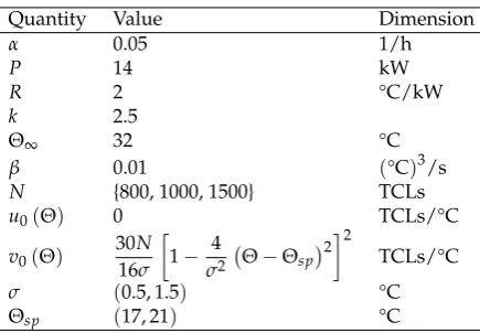
Quantity Value Dimension
α 0.05 1/h
P 14 kW
R 2 °C/kW
k 2.5
Θ∞ 32 °C
β 0.01 (°C)3/s
N {800, 1000, 1500} TCLs
u0(Θ) 0 TCLs/°C
v0(Θ)
30N
16σ
1− 4
σ2 Θ
−Θsp2
2
TCLs/°C
σ (0.5, 1.5) °C
Θsp (17, 21) °C
Table 1.Values of inputs used during simulation
Numerical evaluation ofGij,i,j =1, 2 shows that for the values of parameters represented in
Table1, there always exists a constantCsuch that (16) holds. Therefore, Theorem1is valid and (17) holds. Moreover, it has been observed that for these values, sufficient condition (18) holds implying that the diffusive model above is approximate controllable.
that for fixedσ∈[0.5, 1.5],κdecreases whenΘspincreases in[17, 21]. Therefore, the global minimum ofκ is achieved at Θsp,σ = (21, 0.5). Figure1expresses the behavior of the minimal aggregate consumption against the number of TCLs whenκ0= 1
20max≤t≤Tκ(t). As it is expected,κincreases with
increase ofN. It is also seen from Figure1that as time increases, the minimal aggregate consumption stabilizes around correspondingκ0.
N=800, 1000, 1500
0
2
4
6
8
10
0
500
1000
1500
2000
2500
3000
t
κ
Figure 1.The minimal aggregate power consumption against time forN=800, 1000 and 1500 TCLs
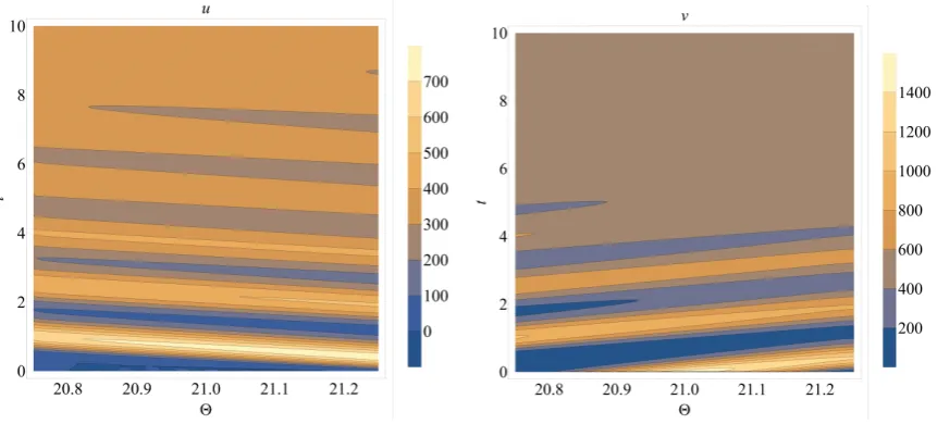
Now let us examine the corresponding solution(u,v). In the contour plots below (Figures 2-4), dark blue regions correspond to near-zero values and the lighter the color of the domain, the higher the corresponding value. ForN = 800, as Figure2shows, fort < 1, in the whole range of
Θ∈[Θmin,Θmax],uis in the dark blue region meaning that the density of TCLs in the on state is low. A similar region occurs neart=2. In between these regions,uapproaches its maximal value in the range ofΘ∈[20.2,Θmax]. Then, the values ofuoscillate between lower and higher values until it is stabilized near ˜u=400 fort≥9. A similar behavior is observed also forvwith the difference thatvis stabilized near ˜v=500 TCLs/°C much earlier, fort≥5.
Figure 2.Contour plots of the distributionsuandvforN=800
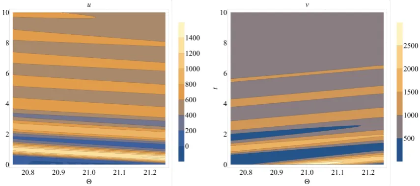
Figure 3.Contour plots of the distributionsuandvforN=1000
Figure 4.Contour plots of the distributionsuandvforN=1500
5. Conclusions
A diffusive behavior in modelling of smart grids of TCLs has been observed recently. The diffusion naturally affects the aggregate power consumption which is a very important criterion in estimating the efficiency of any smart grid of TCLs. In this paper, we consider the controllability property of the diffusive model of TCLs described by a one-dimensional diffusion equation with variable coefficients. The analysis of the governing system is sophisticated by the fact that the system is coupled through the boundary conditions. Involving the Melnikov method for numerical computation of the corresponding Green’s matrix, we derive a sufficient condition for approximate controllability of the grid providing minimal aggregate power consumption. The set-point value and the bandwidth of the temperature act as control parameters.
Acknowledgments:The work of the first author is supported by the School of Mechatronics Engineering and Automation, Shanghai University, China. The work of the second author is supported by State Administration of Foreign Experts Affairs of China.
Conflicts of Interest:Declare conflicts of interest or state “The authors declare no conflict of interest.”.
References
1. Moura S.; Ruiz V.; Bendsten J. Modeling heterogeneous populations of thermostatically controlled loads using diffusion-advection PDEs, ASME Dynamic Systems and Control Conference, ASME, Palo Alto, California, USA, 2013, p. V002T23A001.
2. Sinitsyn, N.A.; Kundu, S.; Backhaus, S. Safe protocols for generating power pulses with heterogeneous populations of thermostatically controlled loads. Energy Conversion and Management 2013, 67, 297–308. 3. Moura, S.; Bendtsen, J.; Ruiz, V. Parameter identification of aggregated thermostatically controlled loads for
smart grids using PDE techniques. International Journal of Control 2014, 87, 1373–1386.
4. Ghaffari, A.; Moura, S.; Krsti´c, M. Modeling, Control, and Stability Analysis of Heterogeneous Thermostatically Controlled Load Populations Using Partial Differential Equations. J. Dyn. Sys., Meas., Control 2015, 137, 101009-101009–9.
5. Kazmi H.; Suykens J.; Balint A.; Driesen J. Multi-agent reinforcement learning for modeling and control of thermostatically controlled loads. Applied Energy 2019, 238, 1022–1035.
6. Ding, Y.; Cui, W.; Zhang, S.; Hui, H.; Qiu, Y.; Song, Y. Multi-state operating reserve model of aggregate thermostatically-controlled-loads for power system short-term reliability evaluation. Applied Energy 2019, 241, 46–58.
7. Eissa, M.M.; Ali, A.A.; Abdel-Latif, K.M.; Al-Kady, A.F. A frequency control technique based on decision tree concept by managing thermostatically controllable loads at smart grids. International Journal of Electrical Power & Energy Systems 2019, 108, 40–51.
8. Bao, Y.-Q.; Chen, P.-P.; Zhu, X.-M.; Hu, M.-Q. The extended 2-dimensional state-queuing model for the thermostatically controlled loads. International Journal of Electrical Power & Energy Systems 2019, 105, 323–329.
9. Perfumo, C.; Kofman, E.; Braslavsky, J.H.; Ward, J.K. Load management: Model-based control of aggregate power for populations of thermostatically controlled loads. Energy Conversion and Management 2012, 55, 36–48.
10. Malhame R.; Chong C. Electric load model synthesis by diffusion approximation of a high-order hybrid-state stochastic system. IEEE Transactions on Automatic Control 1985, 30, 854–860.
11. Callaway, D.S. Tapping the energy storage potential in electric loads to deliver load following and regulation, with application to wind energy. Energy Conversion and Management 2009, 50, 1389–1400.
12. Bashash, S.; Fathy, H.K. Modeling and Control of Aggregate Air Conditioning Loads for Robust Renewable Power Management. IEEE Transactions on Control Systems Technology 2013, 21, 1318–1327.
13. Avetisyan A. S.; Khurshudyan As. Zh. Controllability of Dynamic Systems: The Green’s Function Approach. Cambridge Scholars Publishers, Cambridge, 2018.