Algorithm for Solving an Optimization Problem
for the Temperature Distribution on a Plate
A. Ayriyan1,a, E.E. Donets1, H. Grigorian1,2, N. Kolkovska3, and A. Lebedev1,4
1Joint Institute for Nuclear Research, Joliot-Curie 6, 141980 Dubna, Moscow Region, Russia 2Yerevan State University, Alek Manyukyan 1, 0025 Yerevan, Republic of Armenia
3Institute of Mathematics and Informatics of BAS, Acad. Georgi Bonchev 8, 1113 Sofia, Bulgaria 4GSI Helmholtzzentrum für Schwerionenforschung, Planckstraße 1, 64291 Darmstadt, Germany
Abstract. The work describes the maximization problem regarding the heating of an area on the surface of a thin plate within a given temperature range. The solution of the problem is applied to ion injectors. The given temperature range corresponds to the required pressure of a saturated gas comprising evaporated atoms of the plate material. In order to find the solution, a one-parameter optimization problem was formulated and implemented leading to the optimization of the plate specific geometry. It was shown that a heated area can be increased up to 23.5% in comparison with a regular rectangle form of a given plate configuration.
1 Introduction
The work describes the maximization problem regarding heating of an area on the surface of a thin plate within a given temperature range. The plate serves for injecting the working species (atoms of the plate material evaporated from its surface) into the working space of an ion source [1]. The plate is heated by the flux of the electric current passing through it. The injection starts when the temperature reaches the required value depending on the material of the plate. The temperature range and the working area of the surface respectively are defined by the required pressure of a saturated vapor above the surface of the plate.
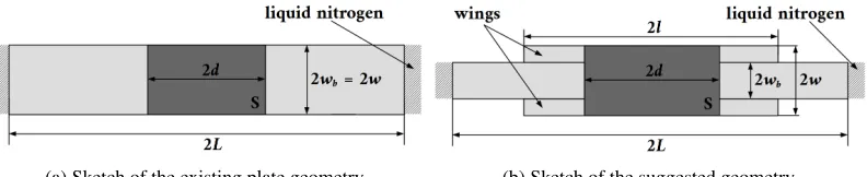
In this work a model of the plate and a one-parameter variation of its geometry are discussed (see figure 1). In the existing technical device the plate has a rectangular form (figure 1a). In order to maximize the working area on its surface we suggested to change the geometry in the following way. A new shape has been derived from the regular one by the removal of rectangular parts from the corners. Thus rectangular wing-like structures (further referenced aswings) appear on the both sides of the plate (figure 1b) with their length being left as a free parameter. Our simulations have shown that the working area of the plate has approximately a rectangular shape for the used set of parameters. The shape of the plate has been optimized by varying the length of these wings in order to reach a maximum working area. The procedure has been applied under the condition that the highest temperature has to be significantly less than the melting temperature of the plate material.
ae-mail: [email protected]
(a) Sketch of the existing plate geometry. (b) Sketch of the suggested geometry.
Figure 1: The geometry of the plate. Here 2Lis the length of the plate, 2wis the width of the plate, 2l is the length of the wings, 2wbis the width without wings,S is the working area of the plate surface
heated to the required temperatures, 2d is the length of the working area. Left and right sides are connected to the temperature terminal.
2 Main Equation and Conditions
The stationary temperature distribution in the plate is modelled by the equation [2]:
∂ ∂x
λ(T)∂T
∂x
+∂∂ z
λ(T)∂T
∂z
+I2χ(T) S2
C
=0, (1)
where the thermal conductivityλ(T) and the resistivityχ(T) depend non-linearly on a sought-after function (temperature),SCis the cross-sectional area, andIis the electric current.
Due to the symmetry at the middle of the plate along thex- andz- axes, solving the problem on a quarter of the full domain is sufficient (see figure 2):
Figure 2:Ω– domain of simulations. The boundary conditions can be taken as following:
⎧⎪⎪⎪ ⎨ ⎪⎪⎪⎩
∂T
∂n =0 if (x,z)∈∂Ω\{(x,z)|z=L}, T =T0 if (x,z)∈ {(x,z)|z=L}.
(2)
The right side of the plate is connected to the tempera-ture terminal withT0 =78 K. At the boundaries of the
domain the temperature gradient vanishes: along thex- andz- axes because of the symmetry and at the other points because the plate is placed inside the vacuum chamber.
The problem (1)–(2) can be solved by various methods. We have chosen the method deriving the solution of the elliptic equation (1) as a stationary solution of the parabolic one (3):
ρ(T)cV(T)∂
T
∂t =
∂ ∂x
λ(T)∂T
∂x
+∂∂ z
λ(T)∂T
∂z
+I2X(T), (3)
here the density isρ(T), the heat capacity iscV(T), andX(T)=χ(T)/S2C. The solution of the elliptic
equation (1) is the stationary solution of the heat equation (3). In order to solve the equation (3) we have assumed the initial condition:
T =T0 ∀(x,z)∈Ω. (4)
3 Formulation of the Optimization Problem
Figure 3: A typical temperature profile versuszfor different lengths of the wings atx=0. The dashed lines correspond to Tlow=678 K andThigh=778 K. The size of the working area is proportional tod.
Thus the maximum of the working area is reached for the maximum ofd. Note that the width of the plate, 2w, is constant. It reaches the maximum possible value following from the technical requirements. The relation
wb/wis fixed. Being dependent on the semilength of the
wingsl(figure 3) for the given temperatureTlow,dis the solution of the following equation forz:
T(x=0,z;l)−Tlow =0, (5) when we choose the source coefficientI(electrical cur-rent) corresponding to the maximum temperature con-straint.
Therefore, the maximum of the working surface area S corresponds to the maximum ofd(l):
d(l∗)=max
0≤l≤L|d(l)|. (6)
The solution of the optimization problem requires repeated solutions of the heat conduction prob-lem (2)–(4).
4 Numerical Algorithms
4.1 Solving the Direct Problem
The finite difference method has been chosen to solve the heat conduction problem (2)–(4):
ρi,jcV i,j
Ti,j−Ti,j
τ =
Λ
x Ti,j
+
Λ
z Ti,j+I2X
i,j, (7)
⎧⎪⎪⎪ ⎪⎨ ⎪⎪⎪⎪⎩
Λ
x[Ti,j]= 1i
λi+1 2,j
Ti+1,j−Ti,j
hi+1 −λi−12,j
Ti,j−Ti−1,j
hi
,
Λ
z[Ti,j]=η1j
λi,j+1 2
Ti,j+1−Ti,j
ηj+1 −λi,j−12
Ti,j−Ti,j−1 ηj
, (8)
wherei=1. . .Nj−1, j=1. . .Mi−1,hi=xi−xi−1,ηj=zj−zj−1,i=(hi+1+hi)/2,
ηj= ηj+1+ηj
/2,Ti,j=T(xi,zj,tk),Ti,j=T(xi,zj,tk+1),cV i,j=cV(Ti,j),Xi,j=X(Ti,j),
λi±1 2,j=λ
Ti,j+Ti±1,j
/2,λi,j±1 2 =λ
Ti,j+Ti,j±1
/2.
The difference scheme (7)–(8) has been solved by the Thomas algorithm [3, 4]:
αi= −
Ci
Bi+Aiαi−1
, βi=
Fi−Aiβi−1 Bi+Aiαi−1
, Ti,j=αiTi+1,j+βi. (9)
The coefficientsAi,Bi,Ci, andFiare defined from the difference equation (7): ⎧⎪⎪⎪ ⎪⎪⎪⎪⎪ ⎪⎪⎪⎪⎪ ⎪⎪⎪⎪⎪ ⎨ ⎪⎪⎪⎪⎪ ⎪⎪⎪⎪⎪ ⎪⎪⎪⎪⎪ ⎪⎪⎪⎩
Ai=−
λi−1 2,j
ihi
,
Bi=
1
i ⎡ ⎢⎢⎢⎢⎣λi−1
2,j hi +
λi+1 2,j hi+1
⎤
⎥⎥⎥⎥⎦+ρi,jτcV i,j,
Ci=−
λi+1 2,j
ihi+1,
Fi=
ρi,jcV i,j
τ Ti,j+ Λz[Ti,j]+I2Xi,j.
The boundary conditions (2) are approximated in the Thomas algorithm as follows:
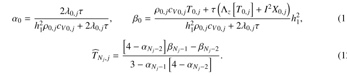
α0 =
2λ0,jτ
h2
1ρ0,jcV0,j+2λ0,jτ
, β0=
ρ0,jcV0,jT0,j+τ Λz
T0,j
+I2X 0,j
h2
1ρ0,jcV0,j+2λ0,jτ
h21, (11)
TNj,j=
4−αNj−2
βNj−1−βNj−2
3−αNj−1
4−αNj−2
. (12)
The initial condition corresponding to (4) isTi,j=T0∀i,j.
The difference scheme (7)–(12) gives a second order approximation of the heat conduction prob-lem (2)–(4) with respect to the spatial steps while first order with respect to time-step. The scheme is unconditionally stable relating to spatial stephiand conditionally stable relating toηj[5]:
τ≤minη
2
j
2 ·min
ρ(T)cV(T)
λ(T)
. (13)
4.2 Algorithm for Solving the Optimization Problem
The algorithm comprises the following steps: 1) the length of the wingsl ∈[0,L] is sampled with a numberNwings; 2) for eachlithe source problem is solved andd(li) is calculated; 3) the value ofl∗is
found according to the maximum value ofd.
The value of the electric currentI varies in the range [0,Imax=500 mA]. IfI reachesImax, the temperature at the central point of the plate exceeds the maximum temperature constraint for all l ∈ [0,L]. In order to find the unique solution existing within the defined range ofI, the bisection method is used.
4.3 Parallel Algorithm
A parallel algorithm for solving the optimization problem was implemented with the usage of Message Passing Interface (MPI) [6]. The main loop of the algorithm 1 (line 2) was parallelized. For eachli
the source problem is solved by a separate parallel process. The parallel algorithm may be executed up toNwingstimes faster in comparison with the sequential one.
5 Results
Numerical results are reported for a plate made of Thulium. Generally, the algorithm has been devel-oped for temperature values depending on the thermal coefficients, but for the present simulations the thermal coefficients [7, 8] are assumed to be constant for the considered temperature range: the con-ductivity isλ=0.169 J/(cm s K), the specific heat iscV =0.16 J/(g K), the density isρ=9.33 g/cm3,
and the ratio of the resistivity to the square of the cross-section area is considered to be the same throughout the whole plateχ/S2
C =103×103Ohm/cm3. The fixed size of the plate wasL =1 cm,
wb=0.05 cm andw=0.125 cm (figure 1b). The sampling numberNwings=10.
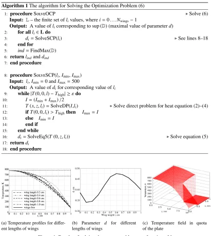
One can see from the figure 4a that the temperature profile is sensitive to the length of the wings. The functiond(l) and the temperature field forl∗ are shown in figures 4b and 4c respectively. The maximumdcorresponds tol∗=0.6 cm.
Fig. 5 illustrates the performance of the parallel algorithm depending on the number of CPUs–np.
The calculations have been carried out on the HybriLIT heterogenius cluster (CPU – Intel Xeon E5-2695). Fig. 5a shows the calculation timetnp, Fig. 5b – the speedup of calculationst1/tnp, and Fig. 5c
– the efficiency of the parallelizationt1/ np×tnp
Algorithm 1The algorithm for Solving the Optimization Problem (6)
1: procedureSolveOCP Solve (6)
Input: L– the finite set oflivalues, wherei=0. . .Nwings−1
Output: A value oflicorresponding to sup (D) (maximal value of parameterd)
2: for allli∈L do
3: di=SolveSCP(li) See lines 8–18
4: end for
5: ind=FindMax(D) 6: returnlindanddind
7: end procedure
8: procedureSolveSCP(li,Imin,Imax) Input: li,Imin=0 andImax=500
Output: A value ofdifor corresponding value ofli
9: while|T(0,0,l)−Thigh| ≥εdo
10: I=(Imin+Imax)/2
11: T(x,z,li)=SolveDP(I,li) Solve direct problem for heat equation (2)–(4)
12: ifT(0,0,li)>Thighthen Imax=I
13: else Imin=I
14: end if
15: end while
16: di=SolveEq5(T(0,z,li)) Solve equation (5)
17: returndi
18: end procedure
(a) Temperature profiles for diff er-ent lengths of wings
(b) Parameter d for different lengths of wings
(c) Temperature field in quota of the plate
Figure 4: Results of solving the source problem as a function ofl
6 Summary and Conclusion
(a) Calculation timetnpin min (b) Speedup:t1/tnp (c) Efficiency:t1/ np×tnp
Figure 5: Results of the parallel algorithm: time, speedup and efficiency of calculations in dependence of number of processors –np
The optimal geometry of the plate has been found (l∗=0.6 cm). This allowed an increase of the working area up to 23.5% in comparison with the one of the regular plate. The value of the electric current corresponding to the maximum working area has been found to be equal toI=385 mA.
Acknowledgements
The study is partially supported by RFBR according to the projects No. 14-01-00628 and No. 14-01-31227. Au-thors thank Edik Ayryan (JINR) for permanent interest in this research and worthwhile discussions, and S. Lebe-dev (JINR & Giessen University) for helpful remarks.
References
[1] D.E. Donets, E.D. Donets, E.E Donets, V.V Salnikov, V.B. Shutov, Journal of Instrumentation5, C09001 (2010)
[2] A.A. Samarskii, P.N. Vabishchevich,Computational Heat Transfer, (Volume 1, John Wiley & Sons Ltd., Chichester, England, 1995)
[3] L.H. Thomas,Elliptic Problems in Linear Differential Equations over a Network (Watson Sci. Comput. Lab Report, Columbia University, New York, 1949)
[4] W.H. Press, S.A. Teukolsky, W.T. Vetterling, B.P. Flannery,Numerical Recipes, third ed. (Cam-bridge University Press, New York, 2007)
[5] N.N. Yanenko,Fractional step methods for solution of multidimensional problems of mathemati-cal physics(Nauka, Moscow, 1967) (in russian)
[6] The Open MPI developer community, http://www.open-mpi.org/(11/06/2015)
[7] I.S. Grigoreva, E.Z. Meylihova, Physical quantities. Handbook (Energoatomizdat, Moscow, 1981)