Probabilistic, features-based object recognition

(1)

Thesis by

Pierre Moreels

In Partial Fulfillment of the Requirements

for the Degree of

Doctor of Philosophy

California Institute of Technology

Pasadena, California

2008

(2)

c

2008

Pierre Moreels

(3)

To my mother,

(4)

(5)

Acknowledgements

First, I wish to thank my thesis advisor, Professor Pietro Perona, for all his help and advice during

my stay at Caltech. Thanks to Pietro, I have enjoyed all these years of PhD research, and hope to

continue working in the field of computer vision.

I wish to thank Pr. Yaser Abu-Mostafa, Pr. Christof Koch, Dr. Larry Matthies and Dr. Baback

Moghaddam, for accepting to be on my thesis defense committee.

I wish to thank Francois Fleuret, Donald Geman, David Lowe, Mario Munich, Michel

Pain-davoine, Jean Pallo, Josiane Zerubia and Andrew Zissermann for very fruitful discussions and

useful suggestions for my research.

I wish to thank all my lab-mates from the Vision lab. Anelia, very nice behind her apparent

bad mood. Claudio, always ready to help for computer-related issues. Marco, the reference for

any math- or manga- related question. Fei Fei and Rob, always full of energy. Seigo, with whom

I enjoyed countless japanese dinners and surfing days. Lihi, whose ideas were always right. The

new lab-members, Greg, Merrielle and Ryan, full of enthusiasm. I started recently to collaborate

with my office-mate and friend Alex Holub, working with him has been very enjoyable, I hope we

will keep doing research together.

(6)

days, windy days, rainy days, all of these are good memories.

I wish to thank Jean-Yves Bouguet, with whom I worked at Intel during one happy summer,

Susan Smrekar, who gave me the chance to work with her at JPL, and Chris Assad, Jay Hanan and

Michael Maire, for collaborating with me on various projects.

I wish to thank my parents and sisters. My parents’ advice was the reason I came to California,

initially to work for one-year at JPL. My parents were always extremely supportive and of good

advice. Sadly, the illness took my mother before she could come to my graduation.

Last, I wish to thank my girlfriend Chihiro. During all these years she waited patiently,

enjoy-ing the few moments of happiness when we could see each other, but livenjoy-ing far apart most of the

year. The day we met was so many years ago that I can barely remember, and I hope we will spend

(7)

Abstract

Object recognition is of fundamental importance in computer vision. In a few years, pedestrian

detection, car detection, and more generally scene recognition will likely be reliable enough to

allow fully-automated car navigation, and the human driver will be relegated to the back seat to sip

his coffee.

In this thesis we are interested in recognizing individual objects and categories. In order to

reduce the volume of information one has to process, images are characterized by sets of features.

These features, also called interest points, are targeted at image locations with high local

infor-mation content. Various systems for detecting interest points and for describing the local image

appearance near these points, have been proposed in the last two decades. We investigate which

combinations from this plethora of detectors and descriptors, are most suited for object recognition

tasks.

On to the problem of object recognition, we are first interested in recognizing individual

ob-jects. In a few years, one can imagine that customers in shops, will take with their cell phone

a picture of a product that looks interesting, send it to a remote server with a huge database of

individual objects, and get back information about that specific product. We propose a system for

(8)

of the recognition process are translated into principled probabilistic terms, which allows us to

outperform a state-of-the-art commercial system for individual recognition.

Regarding categories, faces are probably the category that has received the most attention in

computer vision literature. Here we propose a system to recognize images of the same individual

in large databases of images. This can be of high interest when looking for images of a given

person over the internet. Our method’s advantage is that it works on real-world images, as opposed

to the face databases from the literature, collected in laboratories with controlled lighting, pose and

background conditions.

Finally, we are interested in recognition of object categories in general. Using support vector

machines for the classification task, we propose a features-based kernel that improves recognition

(9)

Chapter 1

(16)

(17)

Learning from examples of seen objects, and being able to recognize these objects in a new

environment, is one great capability of the human visual system and the human brain. Despite

tremendous progress in the recent computer vision literature, the performance of state-of-the-art

software is still far behind human performance.

Several types of tasks are of interest in object recognition. The first one, individual object

recognition, consists of identifying the same exact object in training and test images. One might

be interested in finding e.g. the same exact brand logo, the same exact building, or the same exact

person. In the past, this problem has been addressed in terms of registering a query image to the

best-matching image from the database. Other groups viewed this as a stereo vision problem with

wide base-line. In recent studies, the query scenes deviate from these studies as they are allowed to

contain more than one object from the database. Besides, image scenes do not only contain objects

of interest (foreground), but also a background part. One needs to discriminate between both,

and not only register the foreground part between pairs of images, but also be able to discard the

background. Some applications of individual object recognition available on a commercial basis

include fingerprint or iris identification systems, used as access code as an alternative to passwords.

The second task in object recognition is category recognition, i.e. recognizing that an image

contains a person without identifying which specific person, or a plant without identifying exactly

what type of plant. This task has received a lot of interest in recent years, with constant progress

of the recognition performance on data-sets that have become standard, like the “Caltech-101”.

The category that has seen the highest number of studies is the Face category, so that recently,

commercial digital cameras capable of face recognition in order to improve focus accuracy, or

(18)

appear on the market.

A transversal, but fundamental issue, is how to represent images. While many systems use raw

image information and feed it to the recognition system (e.g. neural-network based applications),

a recently popular approach - which we will adopt in this thesis - is to represent the image via

points of interest, or features. These points of interest characterize the image by a set of

privi-leged locations. The local image appearance or geometry around these locations is then encoded

in a descriptor, and the set of descriptors is used to represent the image. The advantage of this

representation, is to reduce the amount of information that needs to be processed in an image, by

focusing only on a subset of most salient regions. Besides, depending on the encoding used to

rep-resent the local appearance or geometry, one might gain invariance with respect to nuisances like

illumination change, rotation or scaling, affine or projective transformations... One limitation of

this approach is that one has to be careful with regard to the locations selected as points of interest.

For example, while a uniform sky has no salient points, it might be useful to still assign features to

it, when addressing the problem of scene recognition. Ultimately, if infinite computational power

was available, it would be best to characterize images using dense grids of points of interest.

This thesis is organized as follows:

The second chapter investigates which combinations of features detectors and features

descrip-tors are best suited for use in object recognition tasks. A number of detecdescrip-tors and descripdescrip-tors have

been proposed in the past two decades. The literature on features contains comparison studies,

but they have all focused on flat scenes, as ground truth regarding pairs of matching features is

easy to obtain. As a result, features were reported to have an unrealistically high stability across

(19)

triplets of images of 3D objects. The features obtained from various combinations of detectors and

descriptors are matched using this system, to evaluate how stable features are across viewpoints.

The third chapter focuses on individual object recognition. We address the detection problem,

which aims at identifying the objects from the database that are present in a query scene, along

with their location and pose. Motivated by recent studies on coarse-to-fine recognition systems,

we use a cascade of simple detectors, organized from coarse resolution to fine resolution, that filter

quickly through the space of possible hypotheses. Each step is interpreted with a probabilistic

model - this allows us to select parameters automatically rather than tuning them manually, and

provides hypotheses scores in order to decide if hypotheses should be accepted or rejected.

The fourth chapter is also interested in individual objects, for the specific case of faces. We

want to identify the images of a same person, in sets of images that contain numerous irrelevant

faces as well. We characterize face images by sets of features, and investigate which features are

most relevant for the retrieval task. We also learn a distance metric in face-space, that optimizes

the quantity of interest: distances between images of a same person need to be as small as possible,

while distances between images of unrelated persons should be large.

Finally, the fifth chapter looks at the classification problem for object categories. We build

upon the successful pyramid-match kernel - a features-based histogram-type of kernel that was

recently designed and combined with support vector machines, for the task of object classification.

We propose a principled, broader family of kernels, and show that they improve performance

(20)

(21)

Chapter 2

(22)

(23)

2.1

Abstract

We explore the performance of a number of popular feature detectors and descriptors in matching 3D object features across viewpoints and lighting conditions. To this end we design a method, based on intersecting epipolar constraints, for providing ground truth correspondence automati-cally. These correspondences are based purely on geometric information, and do not rely on the choice of a specific feature appearance descriptor. We test detector-descriptor combinations on a database of100objects viewed from144calibrated viewpoints under three different lighting con-ditions. We find that the combination of Hessian-affine feature finder and SIFT features is most robust to viewpoint change. Harris-affine combined with SIFT and Hessian-affine combined with shape context descriptors were best respectively for lighting change and change in camera focal length. We also find that no detector-descriptor combination performs well with viewpoint changes of more than 25–30◦.

2.2

Introduction

Detecting and matching specific features across different images has been shown to be useful for a diverse set of visual tasks including stereoscopic vision [TG00, ea02b], vision-based simulta-neous localization and mapping (SLAM) for autonomous vehicles [SLL02, Low04], mosaicking images [BL03], and recognizing objects [SM97, Low04]. This operation typically involves three distinct steps. First a ‘feature detector’ identifies a set of image locations presenting rich visual information and whose spatial location is well defined. The spatial extent or ‘scale’ of the fea-ture may also be identified in this first step, as well as the local shape near the detected location [MS02, ea02b, TG00, TG04]. The second step is ‘description’: a vector characterizing local visual appearance is computed from the image near the nominal location of the feature. ‘Matching’ is the third step: a given feature is associated with one or more features in other images. Important aspects of matching are metrics and criteria to decide whether two features should be associated, and data structures and algorithms for matching efficiently.

(24)

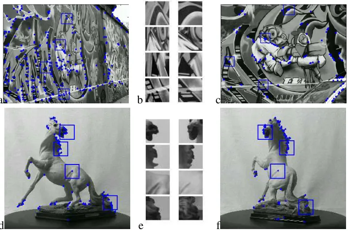
a b c

d e f

Figure 2.1: (Top row) Large (≈ 50◦) viewpoint change for a flat scene. Many interest points can be

matched after the transformation. The appearance change is modeled by an affine transformation. b) shows four40 _×40 patches before and after viewpoint change — images courtesy of K.Mikolajczyk. (Bottom

row) Similar 50◦ viewpoint change for a 3D scene. Many visually salient features are associated with

locations where the 3D surface is irregular or near boundaries. The local geometric structure of the image around these features varies rapidly with viewing direction changes, which makes matching features more challenging because of occlusion and changes in appearance. In particular, the appearance of the patches shown in e) varies significantly with the change in viewpoint. This change is difficult to model.

image, and will match them reliably across different views of the same scene/object. Critical is-sues in detection, description, and matching are robustness with respect to viewpoint and lighting changes, the number of features detected in a typical image, the frequency of false alarms and mis-matches, and the computational cost of each step. Different applications weigh these requirements differently. For example, viewpoint changes more significantly in object recognition, SLAM, and wide-baseline stereo than in image mosaicking, while the frequency of false matches may be more critical in object recognition, where thousands of potentially matching images are considered, rather than in wide-baseline stereo and mosaicking where only few images are present.

(25)

systems. Which combination should be used in a given application? A couple of studies explore this question. Schmid [SM97] characterized and compared the performance of several features detectors. Recently, Mikolajczik and Schmid [MS05] focused primarily on the descriptor stage. For a chosen detector, the performance of a number of descriptors was assessed. These evaluations of interest point operators and feature descriptors, have relied on the use of images of flat scenes, or in some cases synthetic images. The reason is that in these special cases the transformation between pairs of images can be computed easily, which is convenient to establish ground truth.

However, the relative performance of various detectors can change when switching from planar scenes to 3D images (see Figures 2.1, 2.17, and [FB04]). Features detected in an image are generated in part by surface markings, and in part by the geometric shape of the object. The former are often associated with smooth surfaces, they are usually located far from object boundaries and have been shown to have a high stability across viewpoints [SM97, MS05]. Their deformation may be modeled by an affine transformation, hence the development of affine-invariant detectors [LG97, MS02, SZ01, TG00, TG04]. The latter are associated with high surface curvature and are located near edges, corners, and folds of the object. Due to self-occlusion and complexity of local shape, these features have a much lower stability with respect to viewpoint change. It is difficult to model their deformation without a full 3D model of the shape.

The present study generalizes the analyses in [SM97, KS04, MS05] to 3D scenes.1 _We eval-uate the performance of feature detectors and descriptors for images of 3D objects viewed under different viewpoint, lighting, and scale conditions. To this effect, we collected a database of 100 objects viewed from 144 different calibrated viewpoints under 3 lighting conditions. We also de-veloped a practical and accurate method for establishing automatically ground truth in images of 3D scenes. Unlike [FB04], ground truth is established using geometric constraints only, so that the feature/descriptor evaluation is not biased by the choice of a specific descriptor and appearance-based matches. Besides, our method is fully automated, so that the evaluation can be performed on a large-scale database, rather than on a handful of images as in [MS05, FB04].

Another novel aspect is the use of a metric for accepting/rejecting feature matches due to Lowe [Low04]; it is based on the ratio of the distance of a given feature from its best match

(26)

vs. the distance to the second-best match. This metric has been shown to perform better than the traditional ‘distance-to-best-match’.

Section 2.3 presents the previous work on evaluation of features detectors and descriptors. In Section 2.4 we describe the geometrical considerations which allow us to construct automatically a ground truth for our experiments. Section 2.5 presents our laboratory setup and the database of images we collected. Section 2.6 describes the decision process used in order to assess perfor-mances of detectors and descriptors. Section 2.7 presents the experiments. Section 2.8 contains our conclusions.

2.3

Previous work

The first extensive study of features stability depending on the feature detector being used, was performed by Schmid and Mohr [SMB00]. The database consisted of images of drawings and paintings photographed from a number of viewpoints. The authors extracted and matched interest points across pairs of views. The different views were generated by rotating and moving the camera as well as by varying the illumination. Since all scenes were planar, the transformation between two images taken from different viewpoints was a homography. Ground truth, i.e., the homography between pairs of views, was computed from a grid of artificial points projected onto the paintings. The authors measured the performance by the repeatability rate, i.e., the percentage of locations selected as features in two images.

Mikolajczyk et al. [ea05c] performed a similar study of affine-invariant features detectors. This time, most images of the database consisted of natural scenes. However, the scenes were either planar (e.g., graffiti on a wall), or viewed from a large distance, such that the scene appeared flat. Therefore the authors could model the ground truth transformation between a pair of views with a homography as was previously done in [SMB00]. This ground truth homography was computed using manually selected correspondences, followed by an automatic computation of the residual homography.

(27)

one could indeed consider a trivial interest point operator that selects every point in the image to be a new feature. The performance of this detector would be excellent in terms of stability of the features location. In particular for planar images such as considered by [ea05c, SMB00], this detector would reach100%stability. This perfect stability still holds if the detector selects a dense grid of points in the image. This argument illustrates the necessity of including the descriptor stage in performance evaluation.

Fraundorfer and Bischof [FB04] compared local detectors on real-world scenes. Ground truth was established in triplets of views. Correspondences were first identified between grids of points sampled densely in two close views: matches were obtained by nearest neighbor search in appear-ance space. The coordinates of pairs of matching points in the first two images, were transferred on the third image via the trifocal tensor. The test scenes used for detector evaluation were piecewise flat (building, office space).

Mikolajczyk and Schmid [MS05] provided a complementary study where the focus was not anymore on the detector stage but on the descriptor, i.e., a vector characterizing the local ance at each detected location. Two interest points were considered a good match if their appear-ance descriptors were closer than a threshold tin appearance space. Matches that were accepted

were compared to ground truth to determine if they were true matches or false alarms. Ground truth was computed as in their previous study [ea05c]. By varying the acceptance thresholdt, the

authors generated recall-precision curves to compare the descriptors. If the value oftis small, the

user is very strict in accepting a match based on appearance, which leads to a high precision but a poor recall. Ift is high, all candidate correspondences are accepted regardless of their

appear-ance. Correct matches are accepted (high recall), as well as lots of false positives, leading to lower precision.

Ke and Sukthankar [KS04] used a similar setup to test their PCA-SIFT descriptor against SIFT. Test features were indexed into a database, the resulting matches were accepted based on a thresh-old t on quality of the appearance match. Ground truth was provided by labeled images, or by

using synthetic data. The thresholdtwas varied to obtain recall-precision curves.

(28)

performance from the performance of the overall system. The integration within a complete recog-nition method has the advantage of computing directly the bottom line performance in recogrecog-nition. However, the scores might depend heavily on the architecture of the recognition system and may not be generalized to other applications such as large baseline stereo, SLAM, and mosaicking.

2.4

Ground truth

In order to evaluate a particular detector-descriptor combination we need to calculate the prob-ability that a feature extracted in a given image can be matched to the corresponding feature in an image of the same object/scene viewed from a different viewpoint. For this to succeed, the feature’s physical location must be visible in both images, the feature detector must detect it in both cases with minimal positional variation, and the descriptor of the features must be sufficiently close. To compute this probability we must have a ground truth telling us if any tentative match between two features is correct or not. Conversely, whenever a feature is detected in one image, we must be able to tell whether in the corresponding location in another image a feature was detected and matched.

We establish ground truth by using epipolar constraints between triplets of calibrated views of the objects. The motivation comes from stereoscopic imagery: if the position of a point is identified in two calibrated images of a same scene, the position in 3D space of the physical point may be computed, and its location may be predicted in any additional calibrated image of the same scene. We distinguish between a reference view (A in figure 2.2 and figure 2.3), a testviewC, and

an auxiliary view B. Given one reference feature fA in the reference image, any feature in _C

that matches the reference feature must satisfy the constraint of belonging to the corresponding reference epipolar line lAC. This excludes most potential matches but not all of them (in our

experiments, typically 5–10 features remain out of 500–1000 features in imageC). We make the

test more stringent by imposing a second constraint. In the auxiliary imageB, an epipolar line lAB is associated to the reference feature _fA. Again, _fA has typically 5–10 potential matches

alonglAB, each of which in turn generates an ‘auxiliary’ epipolar line_lBC

1...10inC. The intersection

of the primary (lAC) and auxiliary (_lBC

(29)

Figure 2.2: Diagram explaining the geometry of our three-cameras arrangement and of the triple epipolar constraint.

Figure 2.3: Example of matching process for one feature.

(30)

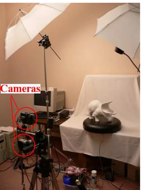
Figure 2.4: Photograph of our laboratory setup. Each object was placed on a computer-controlled turntable which can be rotated with 1/50 degree resolution and 10−5 degree accuracy. Two computer-controlled

cameras imaged the object. The cameras were located10◦ apart with respect to the object. The resolution

of each camera is 3 M pixels. In addition to a neon tube on the ceiling, two photographic spotlights with diffusers are alternatively used to create 3 lighting conditions.

[SW95, HZ00] (transfer using the trifocal tensor avoids the degeneracy of epipolar transfer).

(31)

2.5

Experimental setup

2.5.1

Photographic setup and database

Our acquisition system consists of 2 cameras taking images of objects on a motorized turntable (see figure 2.4). We used inexpensive off-the-shelf Canon Powershot G1 cameras with a 3 MPixel resolution. The highest focal length available on the cameras — 14.6 mm — was used in order to minimize distortion (0.5% pincushion distortion with the 14.6 mm focal length). A change in viewpoint is performed by the rotation of the turntable. The lower camera takes the reference view and the top camera the auxiliary view, then the turntable is rotated and the same lower camera takes the test view. Each acquisition was repeated with 3 different lighting conditions obtained with a combination of photographic spotlights and diffusers. The images were converted to gray-scale using Matlab’s command rgb2gray (keeps luminance, eliminates hue and saturation).

The baseline of our stereo rig, or distance between the reference camera and the auxiliary cam-era, is a trade-off parameter between repeatability and accuracy. On one hand, we would like to set these cameras very close to each other, in order to have a high feature stability (also called repeata-bility rate) between the reference view and the auxiliary view. On the other hand, if the baseline is small the epipolar lines intersect in the test view C with a very shallow angle, which lowers

the accuracy in the computation of the intersection. We chose an angle of10◦ between reference

camera and auxiliary camera; with this choice, the intersection angle between both epipolar lines varied between65◦and₆◦when the rotation of the test view varied between₅◦ and₆₀◦.

(32)

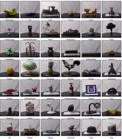
Bannanas Car Car2 Conch Desk Dog

FlowerLamp GrandfatherClock Horse Motorcycle Robot Rock

TeddyBear Tricycle Vase Clock EthernetHub Hicama

Pepper Globe Pineapple Rooster Dremel JackStand

Sander SlinkyMonster SprayCan FireExtinguisher Frame Hat

StaplerRx Carton Clamp EggPlant Lamp Mouse

Oil Basket Clipper CupSticks Filter Mug

(33)

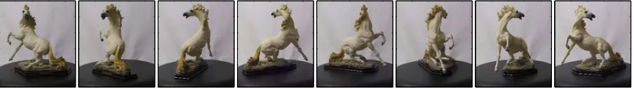
Figure 2.6: Each object was rotated with5◦ increments and photographed at each orientation with both

cameras and three lighting conditions for a total of72_×2_×3 = 432photographs per object. Eight such

photographs (taken every45◦) are shown for one of our objects.

Figure 2.7: Three lighting conditions were generated by turning on a spotlight (with diffuser) located on the left hand side of the object, then a spotlight located on the right hand side, then both. This figure shows 8 photographs for each lighting condition.

2.5.2

Calibration

The calibration images were acquired using a checkerboard pattern. The corners of the checker-board were first identified by the Harris interest point operator, then both cameras were automati-cally calibrated using the calibration routines in Intel’s Open CV library, including the estimation of the radial distortion [Bou99], which was used to map features locations to their exact perspec-tive projection.

(34)

(35)

and selects as features the local maxima of the functiondet(µ)/tr(µ). The second-order moment matrix is a local measure of the variation of the gradient image. It is usually integrated over a small window in order to obtain robustness to noise and to make it a matrix of rank 2 (our implementations used a small5_×5window)

Several other feature detectors use the second-order moment matrix as well. The popular Harris detector [HS88] selects as features the extrema of the saliency map defined bydet(µ)₋0.04_·tr2₍_µ₎.

The Lucas-Tomasi-Kanade feature detector [LK81, ST94] averagesµover a small window around

each pixel, and selects as features the points that maximize the smallest eigenvalue of the resulting matrix. The motivation for these three detectors is to select points where the image intensity has a high variability both in thexand theydirections.

— The Hessian detector [Bea78] is a second-order filter. The saliency measure is here the negative determinant of the matrix of second-order derivatives.

— When the interest point detection is performed at multiple scales, one can combine the locations obtained at all scales.

— The difference-of-Gaussians detector [CP84, Lin94] selects scale-space extrema of the image filtered by a difference of Gaussians. Note that the difference-of-Gaussians filter can be considered as an approximation of a Laplacian filter, i.e. a second-order derivative-based filter.

— The Kadir-Brady detector [KZB04] selects locations where the local entropy has a maximum over scale and where the intensity probability density function varies fastest.

— MSER features [ea02b] are based on a watershed flooding [VS91] process performed on the image intensities. The authors look at the rate of expansion of the segmented regions, as the flooding process is performed. Features are selected at locations of slowest expansion of the catchment basins. This carries the idea of stability to perturbations, since the regions are virtually unchanged over a range of values of the ‘flooding level.’

Characteristic scale — Interest point detectors are typically used at multiple scales obtained

(36)

the Laplacian and the Gaussians. In [Low04], Lowe uses the same difference-of-Gaussians function to detect the interest point locations, i.e., the detector is used to perform a search over scale-space.

Affine invariance— Processes that warp the image locally around the points of interest have

been developed and used by [BG98, LG97, MS02, SZ01] in order to obtain a patch invariant to affine transformations prior to computation of the descriptor. The second-order moment matrix is used as an estimation of the parameters of the local shape around the detected point, i.e., a measure of the local anisotropy of the image. The goal is to deform the shape of the detected region so that it is invariant to affine transformations. The affine rectification process is an iterative warping method that reduces the image’s local second-order moment matrix at the detected feature location to have identical eigenvalues.

Tuytelaars and Van Gool [TG00, TG04] adopt an intensity-based approach. The candidate interest points are local extrema of the intensity. The affine-invariant region around such a point is bounded by the points that are local extrema of a contrast measure along rays emanating from the interest point. In [TG04] they propose another method based on geometry, where the affine-invariant region is extracted by following the edges next to the interest point.

Regarding speed, the detectors based on Gaussian filters and their derivatives (Harris, Hessian, difference-of-Gaussians) are fastest, they can easily be implemented very efficiently using the recursive filters introduced in [VYV98]. The MSER detector [ea02b] has a comparable running time. The detection process typically takes one second or less for a 3 GHz machine on a1024_× 768 image. If one uses the affine rectification process, computation is more expensive, a similar detection takes of the order of 10 seconds. The most expensive detector is the Kadir-Brady detector, which takes of the order of 1 minute on a 800x600 image.

2.5.3.2 Descriptors

(37)

— SIFT features [Low04] are computed from gradient information. Invariance to orientation is obtained by evaluating a main orientation for each feature and rotating the local image according to this orientation prior to the computation of the descriptor. Local appearance is then described by histograms of gradients, which provides a degree of robustness to translation errors.

— PCA-SIFT [KS04] computes a primary orientation similarly to SIFT. Local patches are then projected onto a lower-dimensional space by using PCA analysis.

— Steerable filters [FA91] steer derivatives in a particular direction given the components of the local jet, e.g., steering derivatives in the direction of the gradient makes them invariant to rotation. Scale invariance is achieved by using various filter sizes.

— Differential invariants [SM97] combine local derivatives of the intensity image (up to third-order derivative) into quantities which are invariant with respect to rotation.

- The shape context descriptor [BMP02] is comparable to SIFT, but based on edges. Edges are extracted with the Canny filter, their location and orientation are then quantized into histograms using log-polar coordinates.

The implementations used for the experiments in Section 2.7 were our own for the derivative-based detectors, Lowe’s for the difference-of-Gaussians (includes scale selection in scale-space), and the respective authors’ for MSER and the Kadir detector. Mikolajzyk’s version of the affine rectification process was used. Lowe’s code was used for SIFT, Ke’s for PCA-SIFT, and Mikola-jczyk’s for steerable filters, differential invariants, and shape context.

2.6

Performance evaluation

2.6.1

Matching criteria

The performance of the different combinations of detectors and descriptors was evaluated on a feature matching problem. Each featurefC from a test image_C was appearance-matched against

a large database of features. The nearest neighbor in this database was selected and tentatively matched to the feature. The database contained both features from a reference imageAof the same

(38)

Figure 2.8:( a) Diagram showing the process used to classify feature triplets. ( b) Conceptual shape of the ROC trading off false alarm rate with detection rate. The thresholdTappon distance ratios (Section 2.6.2) is

bounded by[0,1], and the ROC is bounded by the curvep1 +p2 = 1.

larger number (105) of features from unrelated images. Using this large database replicates the

matching process in object/class recognition applications, where incorrect pairs can arise from matching features to wrong images.

The diagram in figure 2.8-(a) shows the decision strategy. Starting from featurefC from the

test imageC, a candidate match tofCis proposed by selecting the most similar amongst the whole

database of features. The search is performed in appearance space. The feature returned by the search is accepted or rejected (T est#1) based on the distance metric ratio that will be described in Section 2.6.2. The candidate match is accepted only if the ratio lies below a user-defined threshold

(39)

Figure 2.9: A few examples of the 535 irrelevant images that were used to load the feature database. They were obtained from Google by typing ‘things.’ 105 features detected in these images were selected at

random and included in our database.

If the candidate match is accepted based on this appearance test, the next stages aim at val-idating this match. T est#2 checks the identity of the image from which the proposed match is coming. If it comes from the image of an unrelated object, the proposed match cannot correspond to the same physical point. The match is rejected as a false alarm.

T est#3 validates the proposed match based on geometry. The test starts from the proposed matchfAin the reference image, it uses the epipolar constraints described in Section 2.4 and tries

to build a triplet (initial feature — auxiliary feature — proposed match) that verifies all epipolar conditions (one constraint in the auxiliary image and two constraints in the test image). As men-tioned in Section 2.4, typically only zero or one feature from the test image verifies all epipolar constraints generated by a given feature from the reference image. If this feature from the test image is precisely our test featurefC, the proposed match is declared validated and is accepted. In

the alternative this is a false alarm.

In case no feature was found along the epipolar line in the auxiliary image B, the initial point fC is discarded and doesn’t contribute to any statistics, since our inability to establish a triple

match is not caused by a poor performance of the detector on the target imageC.

(40)

(41)

(42)

The proposed measure compares the distances in appearance of the query point to its best and second-best matches. In figure 2.8 the query feature and its best and second-best matches are denoted by fC, _fA, and _fA1, respectively. The criterion used is the ratio of these two distances,

i.e. d(fC_,fA₎

d(fC_,fA1₎. This ratio characterizes how distinctive a given feature is, and avoids ambiguous

matches. A low value means that the best match performs significantly better than its best con-tender, and is thus likely to be a reliable match. A high value of the distance ratio is obtained when the feature points are clustered in a tight group in appearance space. Those features are not distinctive enough relative to each other. In order to avoid a false alarm it is safer to reject the match.

The distance ratio is a convenient measure for our study, since the range of values it can take is always[0,1]no matter what the choice of descriptor is.

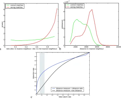
Figure 2.11-(a) shows the resulting distribution of distance ratios conditioning on correct or incorrect matches. The distance ratios statistics were collected during the experiments in Section 2.7. Correct matches and false alarms were identified using the process described in 2.6.1. Figure 2.11-(b) shows the distributions of ‘raw distance to nearest neighbor’ conditioning on correct or incorrect matches. Since distances depend on the chosen descriptor, the descriptor chosen here was SIFT.

Figure 2.11-(c) motivates further the use of the distance ratio by comparing it to raw distance on a classification task. We computed ROC curves on the classification problem ‘correct vs. incorrect match,’ based on the conditional distributions from figures 2.11-(a) and 2.11-(b). The parameter being varied to generate the ROC is the threshold Tapp, which decides if a match is correct or

incorrect. Figure 2.11-(c) displays the results. Depending on the combination detector/descriptor, the operating point chosen for the comparisons in Section 2.7 leads to values ofTappbetween 0.56

(43)

2.6.3

Detection and false alarm rates

As seen in the previous section and figure 2.8, the system can have 3 outcomes. In the first case, the match is rejected based on appearance (probabilityp0). In the second case, the match is accepted

based on distance in appearance space, but the geometry constraints are not verified and ground truth rules the match as incorrect: this is a false alarm (probabilityp1). In the third alternative, the

match verifies both appearance and geometric conditions, this is a correct detection (probability

p2). These probabilities verify p0 + p1 + p2 = 1. The false alarm rate is further normalized

by the number of database features (105). This additional normalization was an arbitrary choice,

motivated by the dependency of the false alarm rate on the size of the database: the larger the database, the higher the risk of obtaining an incorrect match during the appearance-based indexing described in Section 2.6.1. Detection rate and false alarm rate can be written as

f alse alarm rate = #f alse alarms

#attempted matches_·#database (2.2)

detection rate= #detections

#attempted matches. (2.3)

By varying the threshold Tapp on the quality of the appearance match, we obtain a ROC curve

(figure 2.8-(b)). Note that the detection rate does not necessarily reach1whenTappis lowered to

zero since some features will fail Test#2and Test#3on object identity and on geometry.

2.6.4

Number of detected features

For the detectors based on extrema of a saliency map, the thresholdTdet that determines the

min-imum saliency necessary for a region to be considered as a feature, is an important parameter. If many features are accepted, the distinctiveness of each of them might be reduced, as the appearance descriptor of one feature will be similar to the appearance of a feature located only a few pixels away. This causes false alarms during appearance-based indexing of features in the database. Con-versely, ifTdet is set to a high value and only few highly salient regions are accepted as features,

(44)

(45)

2.7

Results and discussion

2.7.1

Viewpoint change

Figure 2.13 shows the detection results when the viewing angle was varied and lighting/scale was held constant. (a)–(h) display results when varying the feature detector for a given image de-scriptor. (a)-(d) display the ROC curves obtained by varying the threshold Tapp in the first step

of the matching process (threshold on distinctiveness of the features’ appearance). The number of features tested is displayed in the legend. (e)-(h) show the detection rate as a function of the viewing angle for a fixed false alarm rate of10−6 was chosen (one false alarm every₁₀attempts

— this is displayed by a gray line in the ROC curves from figures 2.13-2.16). This false alarm rate corresponds to different distance ratio thresholds for each detector/descriptor combination. Those thresholds varied between0.56and0.70(a bit lower than the0.8value chosen by Lowe in [Low04]). Figure 2.14(a)–(b) summarize for each descriptor the detector that performed best.

The Hessian-affine and difference-of-Gaussians detectors performed best consistently with all descriptors. While the absolute performance of the various detectors varies when they are coupled with different descriptors, their rankings vary very little. The combination of Hessian-affine with SIFT and shape context obtained the best overall score, with SIFT slightly ahead. In our graphs the false alarm rate was normalized by the size of the database (105) so that the maximum false alarm

rate was10−5. The PCA-SIFT descriptor is only combined with difference-of-Gaussians, as was

done in [KS04]. PCA-SIFT didn’t seem to outperform SIFT as would be expected from [KS04]. Note that the difference-of-Gaussians detector performed consistently almost as well as Hessian-affine. The difference-of-Gaussians is simpler and faster, this motivates its use in fast recognition systems such as [Low04].

In the stability curves, the fraction of stable features doesn’t reach1whenθ = 0◦. This is due to

several factors: first, triplets can be identified only when the match to the auxiliary image succeeds (see Section 2.4). The 10◦ viewpoint change between reference and auxiliary image prevents a

number of features from being identified in both images.

(46)

(47)

(48)

(49)

(50)

that performs poorly in easy conditions, would outperform all others when matching becomes more difficult. Therefore we believe that matches betweenAandB and betweenAandC are not

independent. In order to avoid any inconsistency, we did not normalize the stability results. Our system is only collecting the most stable features, those that were not only stable betweenAand C, but were successfully matched into triplets.

2.7.3

Flat vs. 3D scenes

As mentioned in Section 2.2, one important motivation for the present study is the difference in terms of stability between texture-generated features extracted from images of flat scenes, and geometry-generated features from 3D scenes. In order to illustrate this stability difference, we performed the same study as in Section 2.7.1, on one hand with 2 images of piecewise flat objects (box of cookies, can of motor oil), on the other hand on two objects with a more irregular surface (toy car, dog). Results are displayed in figure 2.17. As expected, the stability is significantly higher for features extracted from the flat scenes. Note that the stability curves are not as symmetrical with respect to the0◦value as the curves in figures 2.13–2.14. This is due to the fact that here the results

are only averaged over a small number of objects.

One interesting result was that the relative performance of the various combinations detec-tor/descriptor was modified between flat and 3D objects. (e)–(f) display stability results respec-tively for rotations of10◦ and₄₀◦. The fractions of stable features from flat scenes are displayed

on thexaxis, for 3D scenes they are on theyaxis. All combinations lie below the diagonalx=y

since stability is lower for 3D scenes. Some changes in relative performances are highlighted. For example, for flat scenes MSER/SIFT and MSER/shape context performed best, while their perfor-mance was only average for 3D scenes. Conversely, Gaussians/SIFT, difference-of-Gaussians/shape context, and Hessian-affine/shape context, which were the best combinations for 3D scenes, were outperformed on 2D objects.

The dependency of the features stability on the object identity is investigated in figure 2.18. A viewpoint change of10◦was chosen. For each object, the highest fraction of stable features across

(51)

(52)

Figure 2.18: Fraction of stable features for each object of the database, under a fixed viewpoint change of 10◦. For each object, the figure shows the highest fraction of stable features across all investigated

(53)

(54)

by switching the camera’s focal length from 14.6 mm to 7.0 mm. Again, the figure displays only the ‘summary’ panel. Hessian-affine combined with shape context and Harris-affine combined with SIFT obtained the best results.

2.8

Discussion and conclusions

We compared the most popular feature detectors and descriptors on a benchmark designed to as-sess their performance in recognition of 3D objects. In a nutshell: we find that the best overall choice is using an affine-rectified detector [MS02] followed by a SIFT [Low04] or shape-context descriptor [BMP02]. These detectors and descriptor were the best when tested for robustness to change in viewpoint, change in lighting, and change in scale. Amongst detectors, runner-ups are the Hessian-affine detector [MS02], which performed well for viewpoint change and scale change, and the Harris-affine detector [MS02], which performed well for lighting change and scale change. However, the performance of the difference-of-Gaussians detector is close to the affine-rectified de-tectors, while its implementation is simpler and its computation time shorter; therefore we believe it is a good compromise between performance and speed.

Our benchmark differs from previous work from Mikolajczyk and Schmid in that we use a large and heterogeneous collection of 100 3D objects, rather than a set of flat scenes. We also use Lowe’s ratio criterion, rather than absolute distance, in order to establish correspondence in appearance space. This is a more realistic approximation of object recognition. A major difference with their findings is a significantly lower stability of 3D features. Only a small fraction of all features (less than 3%) can be matched for viewpoint changes beyond 30◦. The situation is a bit better when the

goal is stereo-vision or mosaicking (figure 2.14-(c)), where features are matched across a small number of images. Our results on descriptors favor SIFT and shape context descriptors, and are in agreement with [MS05]. However, regarding detectors, not all affine-invariant methods are equivalent as suggested in [ea05c] — e.g., MSER performs poorly on 3D objects, while it is very stable on flat surfaces.

(55)

appear to contain a high proportion of highly textured quasi-flat surfaces (boxes, desktops, building facades, see figure 6 in [FB04]). This hypothesis is supported by the fact that our measurements on piecewise flat objects (figure 2.17) are more consistent with their findings. Another difference with their study is that we establish ground truth correspondence purely geometrically, while they use appearance matching as well, which may bias the evaluation.

(56)

(57)

Chapter 3

(58)

(59)

3.1

Abstract

A coarse-to-fine probabilistic model for detecting objects in images is presented. Objects are com-posed of constellations of features, and features from a same object share the common reference frame of the image in which they are detected. Features’ appearance and pose are modeled by probabilistic distributions, the parameters of which are shared across features in order to allow training from few examples.

In order to avoid an expensive combinatorial search, we propose a coarse-to-fine strategy, in-spired by the work of Lowe [Low99, Low04] and of Geman and collaborators [AGF04, FG01]. Well-established, simple, and inexpensive steps are used as successive refinement blocks that dis-card incorrect matching hypotheses in a cascade. The candidate hypotheses output by our algo-rithm are evaluated by a generative probabilistic model that takes into account each stage of the matching process.

We apply our ideas to the problem of individual object recognition and test our method on several data-sets. We compare with Lowe’s algorithm and demonstrate significantly better perfor-mance.

3.2

Introduction

Recognizing objects in images is perhaps the most challenging problem currently facing machine vision researchers. Much progress has been made in the recent past both in recognizing individual objects [FTG04, Low04], as well as in recognizing object categories [BBM05, FPZ03, LSP06, OFPA04, WWP00]. Other groups have interpreted the problem of individual object recognition and detection as a wide-baseline problem; their work aims at registering pairs of images with each other [FTVG05, ea02b, PZ98, Rot04]. A number of ideas have proven to be key to recent progress. First of all: objects and categories may be represented as collections of features, each

(60)

in the image — if one enforces both mutual position and appearance constraints one may rule out false alarms arising from features detected in random clutter. This provides robustness to occlusion and poor feature detection — even if many model features are missing in the test image, recognition can proceed with the remaining features. Third: very efficient approximate algorithms for matching features in the high dimensional space where the features’ appearance is represented have been discovered [BL97]. Similarly, there exist efficient algorithms for enforcing geometrical constraints [FB81, FG01, Low85]. The combination of these ideas and techniques has given us very efficient and robust object recognition algorithms.

However, much progress still needs to be made to reach levels of performance comparable to those of the human visual system. Error rates are still large on fairly benign benchmark image sets [KSP07, LSP06, MP04, WZFF06]. Furthermore, many classes of objects are still difficult to recognize or discriminate: e.g., objects containing repeated textures (furry teddy bears) and objects with smooth featureless surfaces (plain coffee mugs). In order to overtake some of the current challenges we need to be creative and generate novel image analysis ideas, e.g., new feature types. Another way to make progress is to place our recent discoveries on a firm theoretical footing. Much of what we know is still a ‘bag of tricks’ — we need to understand better the underlying principles in order to improve our designs and take full advantage of what we can learn from the statistics of images.

In this study we focus on recognition of individual objects in complex images. Our goal is to produce a consistent probabilistic interpretation of the recognition system from Lowe [Low99, Low04], one of the most effective techniques we know for individual object recognition. The techniques we use are inspired by the work of Burl [BMW98], Weber [WWP00], and Fergus [FPZ03] on the probabilistic ‘constellation’ model for object categories. We are also inspired by Amit [AGF04] and Fleuret [FG01] and their work on coarse-to-fine searching.

(61)

the test image with very little effort, before analyzing the remaining regions of hypothesis space in greater detail.

Second novel contribution: we introduce a generative probabilistic model that evaluates the hypotheses taking into account each stage of their formation. Regarding parameters estimation, we benefit from a recent study measuring the variation in position and appearance of features in 3D objects imaged under different viewpoints and lighting conditions – various conditional probabilities in our algorithm are therefore based on careful empirical measurements [MP07b].

Third: although this was not the main goal of our study, our experiments show that our new algorithm and probabilistic scoring model, perform substantially better than a state-of-the-art de-tection system developed independently by Lowe [Low99, Low04].

Section 3.3 introduces our generative model. Section 3.4 describes the coarse-to-fine process used to generate hypotheses and sets of features assignments. Sections 3.5 and 3.6 explain in detail the probabilistic model and parameters estimation used to assign a score to the hypotheses. Section 3.7 presents and discusses results, and Section 3.8 contains our conclusions.

3.3

Generative model

3.3.1

Object recognition scenario

Our target scenario consists of recognizing individual objects in complex images [Low99, Low04]. We assume that a number ofknown objectshave been gathered. We collect images of these objects,

the images collected for each object form the modelof this object. The set of models form our

database. In the experiments of Section 3.7 we consider one or few training images per known

object. On the other hand, we are given a query image, which is the photograph of a complex

test composition containing some of the known objects — we call this image the test image. In

(62)

3.3.2

Modeling object images as collections of features

The physical objects photographed in the database and in the test image are represented as a spa-tially deformable collection ofparts [BMW98, FPZ03, FB81, ea93, WWP00, WFKvdM97]. In

images of the objects, these parts are associated to visually distinctivefeatures. In probabilistic

terms, one may model this as the object parts being the cause of visual features, whose loca-tion and appearance is a random variable centered on a nominal localoca-tion and appearance. Fig-ure 3.1-(a) displays the featFig-ures identified by the commonly used difference-of-Gaussians detec-tor [CP84, Lin94, Low04] on several images of the same face. Some features and groups of fea-tures are geometrically consistent with each other across different views of the face, since they are detected repeatedly near the same physical location on the face. On the other hand, since the background is different from one image to the next, the locations of the background features de-tections are unrelated between any two images. Features-based object recognition methods based only on such considerations on pose, have been developed successfully, e.g., by Lowe [Low85] and more recently by Fleuret and Geman [FG01]. In both cases the authors use perceptual grouping of simple features to form objects.

In general, building a recognition system based only on such considerations on pose, is a hard task: one challenge, when we want to put into correspondence features from the database and from the test image, is due to the different number of features generated by the same object in separate images containing it. These different numbers of features are due to differences in lighting conditions and in viewpoint, imaging noise, resolution, or occlusions. For example, an object imaged successively from far and from a close viewpoint, shows more detail in the second picture, thus generating more features.

While pose information is a very useful tool for recognition, additional information is provided by image descriptors which represent the local image texture orappearancenear these points of

(63)

(64)

had good success with a characterization of features that considers appearance only and discards pose information (‘bag of features’ approaches).

In this paper, we will consider both pose and appearance. A feature will be calledstablewhen

it is both found repeatedly near the same physical object part in separate images, and generates descriptors that are very close in appearance space [MP07b]. The features’ pose (location, scale, orientation), along with their appearance description will be all the knowledge that we learn from training images of known objects. In the test image, features’ pose and appearance will be our evidence regarding presence or absence of some of the known objects in the test image.

In a model, the features are caused by parts of the known object or by random background events. In the test image, the features are either caused by a known object present in the test composition, or they originate from objects not present in the training set and from random clutter. The former type of features will be called foreground features, the latter background features.

Clutter features may appear everywhere in the test image, in particular on the footprint of the known objects, these features cannot be matched to the database models. In order to recognize objects in the test image, we need to establish correspondences between test image and database, i.e., identify subsets of the test features as well as subsets of the database features that are both consistent in terms of geometrical structure, and match each other in terms of appearance. Large subsets of corresponding features, and good consistency in pose and appearance, are indicators of the presence of the object in the test image. We will discuss how this may be interpreted in probabilistic terms in Sections 3.5 and 3.6. During the matching process, a fraction pdet of the

database features associated to the objects present in the test image can be associated successfully to corresponding features in the database. Similarly, a fractionpstray of the test image’s background

features are extremely similar in appearance to database images, and form spurious matches that we need to reject.

3.3.3

Probabilistic interpretation of the test image

(65)

(66)

in the test image.

3.4

Hypothesis generation

Ahypothesiscontains the identity of the known objects that are believed to be present in the test

image, along with their pose. In this section we describe the algorithms that are used to generate likely hypotheses, in Sections 3.5–3.6 we will present the probabilistic scoring method used to evaluate hypotheses.

3.4.1

Test image and models

As mentioned in Section 3.3.2, all test compositions and known objects, are represented by collec-tions of distinctive features. In this work we use the popular combination of multi-scale difference-of-Gaussians detector and SIFT descriptor proposed by Lowe [Low04], although a few other op-tions are equally good [ea05c, MS05, MP07b]. We calldatabase of featuresand denote byM the

set of features extracted in images of known objects, and denote byF the set of features extracted

from the test image.

Known objects, in number _M, are indexed by k and denoted by mk (k will appear both as

a subscript and a superscript, but will always denote a known object). The indices i and j are

used respectively for test features and database features: fi denotes the i-th test feature, while

fk

j denotes the j-th feature from the k-th object. The number of features detected in images

of object mk is denoted by nk. For the M known objects, these cardinalities form the vector n ₌ _{_n_k_}_k _{= (}_n₁_...n_M₎. Therefore,_M is a set of sets of features: _M ₌ _{_fk

j}j=1...nk _k₌₁_..._M.

Note: throughout this paper, bold notation will denote vectors.

A special object, denoted bym0, represents the background clutter which generates unwanted

detections. The number of features in the ‘background object’ is not known in advance.

Each feature is described by itspose informationand itsappearance: fi = (Xi,Ai)for a test

feature,fk

j = (Xjk,Akj)for an object feature (see figure 3.3). The pose information is composed

of position informationx, y, scales, and orientationθ in the image. We have_Xi = (xi, yi, si, θi)

for test features, and similarly Xk

(67)

informa-test image

predic ted pose

model

tentative match

Figure 3.3: This figure illustrates the notation related to features. The pink points represent the location where the feature was detected, the blue squares represent the image area that is sampled to compute the appearance descriptors. Model featuref_jkmatches test image featurefiwhen its appearanceAk_j is closest to

Aiin the database. The transformation between the two features’ posesXjkandXipredicts the model’s pose

in the test image. This pose prediction is the building block of the Hough transform described in Section 3.4.2.2.

tion is measured relative to the standard reference frame of the image in which the feature has

been detected. All features extracted from the same image share the same reference frame. The

appearanceinformation associated to a feature is a descriptor characterizing the local image

ap-pearance, or texture, in a region of the image centered at this location. It is denoted byAi for test

featurefi andAkj for database featurefjk.

A hypothesisH is an interpretation of a test image, i.e., a subset of the known objects m ₌

{mk}k together with their posesΘ = {Θk}k. Note that repetitions are allowed since two similar

objects can be present in the test image (e.g., two cans of Pepsi), therefore this is a multiset. In

order to keep a simple terminology, we will nevertheless call this a set. The objects specified by the hypothesis are believed to be present in the test composition, thus ‘causing’ the test. Aposeis a set

of parameters that map a known object onto a corresponding object in the test composition. In this paper we consider affine transformations. Thus, an object’s pose is the affine transformation that maps a database model onto a corresponding object in the test image (see figure 3.3). The number of objects specified present by the hypothesis is denoted by H. A hypothesis can be a no-object

(H = 0), single-object (_H = 1), or multi-objects hypothesis (_H > 1). We will consider first

single-object hypotheses; in Section 3.4.4 we will investigate how to combine them into multiple-objects hypotheses. We denote byH0the special hypothesis that considers no object to be present

(all features are clutter detections).

(68)

present with which pose, i.e., a true hypothesisHtrue.

An assignment vectorV carries complementary information to a hypothesis: it assigns each

feature from the test image to a database feature (in which case we call it a foreground feature)

or to clutter (background feature). Thei-th componentV(i) = (k, j)denotes that the test feature

fi is matched to fjk, j-th feature from thek-th object mk. V(i) = 0denotes the case whenfi is

attributed to clutter.

We also assume that in each test image there is an underlying ground truth regarding the as-signment vector. Features detections in images are triggered by informative parts on the physical objects, both in models and in the test image. The correspondences between parts on the physical objects, and features detected respectively in models and in the test image, are a hidden variable. These correspondences induce a ground truth set of correspondences V_true between features in

models and features in the test image.

3.4.2

Coarse-to-fine hypotheses filtering

Given a test image, our goal is to come up quickly with a likely explanationH. Before we see the

test image, all hypotheses are possible explanations. Since there are very many hypotheses to be considered, our strategy will be to exclude as many as possible from consideration at an early stage. We use a coarse-to-fine strategy inspired by Amit [AGF04] and Fleuret [FG01]. In these lines of work, a same object detector is run several times from a coarse resolution to a fine resolution. At coarse resolution, the detector can exclude quickly large, irrelevant regions of the hypothesis space without exploring them in detail. The disadvantage of using a coarse detector is that it is not able to output a precise hypothesis, but can only tell which large regions of the hypothesis space might contain an object. Next, the regions that triggered this coarse detector are explored again at a finer resolution. This second detection stage rejects more regions of hypothesis space, and focuses more precisely on the relevant locations. The process is repeated several times until the target resolution is reached.

(69)

(70)

(71)

number of matches — defined by a thresholdTk

votes — are considered in the subsequent steps. We

will see