Reflection and Transmission of Waves at the Interface of Perfect Electromagnetic Conductor (PEMC)

REFLECTION AND TRANSMISSION OF WAVES AT THE INTERFACE OF PERFECT ELECTROMAGNETIC CONDUCTOR (PEMC)

I. V. Lindell and A. H. Sihvola Electromagnetics Group

Department of Radio Science and Engineering Helsinki University of Technology

Box 3000, Espoo 02015TKK, Finland

Abstract—Perfect electromagnetic conductor (PEMC) has been introduced as a generalization of both the perfect electric conductor (PEC) and the perfect magnetic conductor (PMC). In the present paper, the basic problem of reflection and transmission of an obliquely incident plane wave at the interface of a PEMC half space or slab is considered. It is found that the field outside the PEMC medium can be uniquely determined but the interior field requires some assumptions to be unique. In particular, definition of the PEMC-medium condition as a limit of a Tellegen-medium condition and extraction of certain virtual fields (metafields) are shown to make the field inside the PEMC medium unique.

1. INTRODUCTION

The concept of perfect electromagnetic conductor (PEMC) has been defined by medium conditions of the form [1, 2]

D=MB, H=−ME, (1) where M is the PEMC admittance parameter, also called the axion parameter by the physicists [3, 4]. The PEMC concept has given rise to numerous studies on the topic [10–14]. In this study, the medium is assumed lossless, whence M is restricted to have real values, positive or negative [5]. In fact, for real M the complex Poynting vector is imaginary,

S= 1 2E×H

∗₌₋M

2 E×E

whence the fields in PEMC do not convey energy. Actually, one can show that the Maxwell energy-stress dyadic [3, 6] vanishes for all possible fields if and only if the medium is PEMC. Thus, there is no energy involved in the fields occupying the PEMC.

The classical perfect electric conductor (PEC) and perfect magnetic conductor (PMC) are two special cases corresponding to the respective parameter values 1/M = 0 andM = 0. For convenience in expressions we can also define the PEMC medium in terms of an angle parameterϑdefined by

M = 1

ηo

tanϑ, ηo =

µo/o. (3)

In this case PEC corresponds toϑ= 0 and PMC to ϑ=±π/2. PEMC can also be defined as a Tellegen medium obeying the medium conditions of the form [1]

D B

=q

M 1

1 1/M

E H

, (4)

in the limit of the parameter|q| → ∞. In fact, the conditions (4) can be expressed in equivalent form as

D−MB= 0, H+ME=D/q, (5) from which we find thatD =MB is exactly satisfied for anyq, while the condition H= −ME will be approached in the limiting process. (4) cannot be inverted, because the determinant of the matrix is zero. However, another similar process can be defined as

E H

=q

1/M −1

−1 M

D B

, (6)

or

H+ME= 0, D−MB=−H/q, (7) which, again, approaches (1) in the limit|q| → ∞.

from and transmission through a planar interface between an isotropic half space and a half space of PEMC medium. A similar problem was studied by Jancewicz [7] for a normally incident wave. Starting from the condition (1), he found that the fields inside the PEMC medium could not be uniquely determined, while the reflected fields of [1, 2] were reproduced. In the present study we approach the same problem with an obliquely incident time-harmonic wave which can be interpreted as a Fourier component of the most general field. For convenience, expressions related to incident and reflected plane waves, although quite well known in the literature [8], will be first derived to introduce the notation used in this paper.

z

ki kr

kz

-kz kx

-kt z

z = 0

µo o ... _{PEM C}

... ... ... ... ... ... ... ... ... ... ... ... ... ... ...

x

∋

→

→ ,

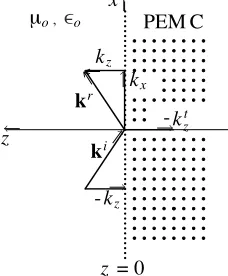
Figure 1. Plane-wave incident upon the interface of PEMC half space creates a transmitted field propagating along the interface with the wave numberkx.

2. REFLECTION FROM A BOUNDARY 2.1. Plane-wave Fields

Let us consider a time-harmonic plane wave incident in the half space

z > 0 to an interface of a second medium at z = 0 which causes a reflected wave. The incident and reflected electric and magnetic fields are assumed to have the form

Ei(r) = Eiexp

−jki·r

, Hi(r) =Hiexp

−jki·r

, (8)

Er(r) = Erexp (−jkr·r), Hr(r) =Hrexp (−jkr·r), (9) where the two wave vectors are defined by

and kx is assumed to be a positive real number. The half spacez >0 is assumed empty, whence the wave-vector components satisfy

k2_z+k2_x=k_o2=ω2µoo. (11)

The Maxwell equations for a plane wave in the source-free regionz >0 have the form

k×E=koηoH, ηok×H=−koE, (12) withηo=

µo/o. Because the electric fields satisfy the orthogonality conditions

ki·Ei = 0, kr·Er= 0, (13) they can be expressed in terms of their components transverse to the

z axis as

Ei = 1

kz

kxuzux+kzIt

·Ei_t, (14)

Er = 1

kz

−kxuzux+kzIt

·Er_t. (15) Vectors transverse touz are defined through the transverse projection dyadic It and denoted by the subscript t as

at=It·a, It=uxux+uyuy. (16) Inserting (8) and (9) in (12), we obtain

ηoHi = 1

kzko ki×

kxuzux+kzIt

·Ei_t, (17)

ηoHr = 1

kzko

kr×−kxuzux+kzIt

·Er_t, (18) whence the relations of the transverse field components can be expressed in the compact form

Hi_t=Yt·Eit, Hrt =−Yt·Ert. (19)

Ytis the free-space admittance dyadic. It can be expressed in the form

Yt= 1

ηo

Jt, (20)

whereJt is the dimensionless dyadic

Jt= 1

kokz

k2_zuxuy−ko2uyux

satisfying

J2_t =−It. (22)

Because of this property, the normalized admittance dyadic Jt resembles the imaginary unit and it creates what is called an almost-complex structure in the space of two-dimensional vectors [3, 9].

2.2. Interface Conditions

Let us assume that the boundary at z = 0 is an interface of another medium occupying the half spacez <0 and the plane wave transmitted through the interface has the form

Et(r) =Etexp−jkt·r, Ht(r) =Htexp−jkt·r. (23) Continuity of the fields along the interface requires that the wave vector be of the form

kt=uxkx+uzktz, (24) where k_zt depends on the medium behind the interface. Continuity of the transverse fields through the interface requires the conditions

Ei_t+Er_t = Et_t, (25)

Jt·(Eit−Ert) = ηoHtt (26)

to be valid.

A relation between the incident and transmitted fields can be found by eliminatingEr_t from (25) and (26):

2Ei_t=Et_t−Jt·ηoHtt. (27) If a linear relation between the transmitted transverse field components is known in the form

Ht_t=Yt_t·Et_t, (28) from (27) the transmitted electric field can be expressed as

Et_t= 2Jt+ηoYtt

₋1

·Jt·Eit. (29) The reflected field can then be found from (25) in the form

Er_t =Rt·Eit, (30) where the reflection dyadic is defined by

Rt=

Jt+ηoYtt

₋1

·Jt−ηoYtt

2.3. Metafields

To consider uniqueness for the fields in the medium behind the interface atz= 0 one may ask whether there could exist fieldsEt

o,Hto,Bto,Dto in the PEMC half space without any sources or fields causing them in the region z > 0. This means that we are looking for fields in the regionz <0 satisfying the conditions

uz×Eto = 0, uz×Hto = 0, (32) uz·Bto = 0, uz·Dto= 0, (33) at the interface z = 0. Existence of such virtual fields or metafields, as they may be called, depends on the medium in the half space

z < 0. For example, in an isotropic medium with permittivity and permeabilityµ, one can easily show that the conditions (32), (33) would lead to vanishing of the field. However, for the PEMC conditions (1) there actually may exist nonzero metafields. For example, assuming the previous exponential dependence on x, the following metafields, derived from an arbitrary scalar function Eo(z), satisfies the interface conditions (32)

Et_o(r) =uzEo(z)e−jkxx_{, H}t

o(r) =−MEto(r). (34) From the Maxwell equations we obtain the other field components,

Bt_o(r) =−uykx

ω Eo(z)e

−jkxx_{, D}t

o(r) =Bto(r)/M, (35) which satisfy (33).

Thus, for any scalar functionEo(r) such a metafield may exist in the PEMC half space without anyone noticing its existence from the outside. Because such a field appears nonphysical, we could extract it from any solution.

2.4. PEMC Interface

The relation (28) depends on the properties of the medium in the half space z <0. For the PEMC half space the medium conditions (1) are also valid for the transverse field components, whence the interface is defined by the admittance dyadic

Yt_t=−MIt. (36)

Inserting in (31) we can expand

Rt=−

Jt+ηoMIt

2

1 + (ηoM)2

= 1−(M ηo)

2

1 + (M ηo)2

It−

2M ηo 1 + (M ηo)2

For example, for PEC corresponding toϑ= 0 andM =∞ we obtain

Rt=−It andErt =−Eit. Expressing

ηoM = tanϑ, (38)

we can represent the reflection dyadic compactly as

Rt= cos 2ϑIt−sin 2ϑJt= exp

−2ϑJt

, (39)

whose validity is based on the Taylor series expansion of the exponential. In the special case of normal incidence, withkz =ko and

Jt=−uz×I, the reflection dyadic (37), (39) coincides with that derived in [1, 2], when the opposite orientation of uz is taken into account.

For general incidence the reflected transverse field becomes

Er_t =Rt·Eit= cos 2ϑEit−sin 2ϑJt·Eit. (40) The total transverse fields at the interface define the transverse component of the transmitted field as

Et_t=Ei_t+Er_t = 2 cosϑexp−ϑJt

·Ei_t, (41) or

Et_t= 2 1 + (M ηo)2

Ei_t−M ηoJt·Eit

. (42)

The magnetic field can be obtained similarly as

ηoHtt=Jt·

Ei_t−Er_t=−2 sinϑexp−Jtϑ

·Ei_t, (43) which equals−ηoMEtt, as expected.

3. FIELDS IN THE PEMC MEDIUM 3.1. PEMC Conditions

Starting from the PEMC conditions (1) does not yield unique transmitted fields, since the two Maxwell equations

components out of 14. From (44) and (45)Dt_z,B_zt can be solved which increases the number of known components to 7. The remaining 7 unknown components, E_zt, H_zt,B_tt,Dt_t and kt_z cannot be solved from (44) and (45). Actually, we only need to know two of the unknowns,

k_zt and, e.g., E_zt, to be able to solve the remaining five from (44) and (45).

It is not much of an improvement to start from the PEMC conditions of the form (6). In fact, eliminatingEtandBt, (45) can be written as

kt×Ht=−ωDt+Ht/q, (46) whence together with (44) this would requireHt/q = 0 and, for finite

q, Ht _{= 0 which eventually would lead to vanishing of all fields. To} avoid that, we must have |q| = ∞ from the start, which means that (6) coincides with (1).

We can try to approach uniqueness by extracting a metafield component from the fields on the physical grounds that a field without a source cannot exist. Since any field of the form (34), (35) is a metafield, we can actually require that the transmitted fields satisfy

uz·Et= 0, uz·Ht= 0. (47) After the metafield extraction there still remains the question about thez dependence of the fields because PEMC allows all possible wave vectors. The most obvious choice would be k_zt = 0. However, if we consider a slab of PEMC instead of the half space, this will cause a problem at the other interface, as will be seen. Thus, kt_z remains an open parameter and no uniqueness is achieved when starting from the conditions (1) or (5).

3.2. Tellegen Conditions

Let us now start from the Tellegen medium conditions (4) and assume a finite value for the parameterq,

Dt = q

Ht+MEt

, (48)

MBt = q

Ht+MEt

. (49)

To simplify the analysis, we temporarily define two auxiliary vectors F,Gby

F= 1

2M(ME+H), G=

1

whence the fields can be expressed as

E = F+G, (51)

H = M(F−G). (52) Inserting these in (44) and (45), the resulting Maxwell equations

Mkt×(F−G) = −2ωqMF, (53)

Mkt×(F+G) = 2ωqMF, (54) can be reduced to

kt×F = 0, (55) kt×G = 2ωqF. (56) Because of the assumptionkx >0 we havekt= 0 and there must exist a scalarα such that

F=αkt. (57)

The second Equation (56) can now be written as

kt×G= 2ωqαkt= 2ωγkt. (58) To avoid fields growing infinite when q → ∞, we must assume that simultaneouslyα→0 so that

γ =qα (59)

remains finite. (58) implies

kt·kt= 0, ⇒ kt=kx(ux+juz), (60) withkt _satisfying

uy×kt=jkt. (61) The other possibilitykt=kx(ux−juz) is ruled out by requiring that the field must not grow exponentially asz→ −∞. Expanding (58) as

uy×

kt×G

=kt(uy·G) = 2jωγkt, (62) we see thatGmust be of the form

The electric and magnetic fields can now be expressed as

Et = F+G= (αkx+β) (ux+juz) + 2jωγuy, (64) Ht = M(F−G) =M(αkx−β) (ux+juz)−2jωM γuy. (65) whence the fields satisfy

Ht+MEt= 2M αkt= 2M γ

q k

t_{. (66)}

Comparing this with (48) and (49), we can identify

Dt= 2M γkt, Bt= 2γkt. (67) Now we can safely letq→ ∞, whence the electric and magnetic fields become

Et→β(ux+juz) + 2jωγuy, (68) Ht→ −M β(ux+juz)−2jωM γuy. (69) The unknown parameters β, γ can be found by comparing the transverse components of Et _{to those obtained from the interface} condition (42), rewritten as

Et_t = 2

kokz(1 + (M ηo)2)

ux

kokzux−M ηokz2uy

+uy

kokzuy+M ηok2oux

·Ei_t. (70)

β =

2koExi −M ηokzEyi

ko(1 + (M ηo)2)

, (71)

γ = kzE i

y+M ηokoExi

jωkz(1 + (M ηo)2₎. (72)

When applying to the normally incident wave with kz →ko,kx → 0, we obtain

β →

2Ei

x−M ηoEyi

1 + (M ηo)2

, (73)

γ → E

i

y+M ηoExi

jω(1 + (M ηo)2₎, (74)

and

Et→ 2 1+(M ηo)2

It+M ηouz×I

·Ei+juz

Ei_x−M ηoEyi

This result contains a discontinuity because theE_ztcomponent depends on the choice of thexaxis: it obtains different values when approaching normal incidence from different directions.

To remove this defect from the solution we again extract the z

components of the Et and Ht fields, because they can be interpreted as metafields (34).

Thus, we obtain the final field expressions

Et(r) = 2e

−jkxx_ekxz

kokz(1+(M ηo)2)

kokzIt+M ηo

k2_ouyux−k2_zuxuy

·Ei, (76)

Ht=− 2M e−

jkxx_ekxz

kokz(1+(M ηo)2)

kokzIt+M ηo

k_o2uyux−kz2uxuy

·Ei, (77)

Bt(r) =kx

ω(ux+juz)×E

t_(r)

= 2kxe

−jkxx_ekxz

ωkokz(1 + (M ηo)2)

kokz(ux+juz)×It−jM ηo

k2_o(ux+juz)ux+k2_zuyuy

·Ei, (78)

Dt(r) =MBt(r). (79)

In this way we have arrived at a unique representation of the fields inside the PEMC half space. For the normal incidence case kx → 0 we see that the Bt and Dt fields vanish while the other fields become constant in the half space,

Et(r)→ 2 1 + (M ηo)2

It+M ηouz×It

·Ei, (80)

Ht(r)→ − 2M 1 + (M ηo)2

It+M ηouz×It

·Ei, (81) as obtained from (75).

3.3. PEC and PMC

For the PMC half space corresponding toM = 0 (76)–(79) become

Et(r) = 2Ei_te−jkxx_ekxz_{, H}t_{= 0, (82)} Bt(r) = 2kx

ω (ux+juz)×E

i

te−jkxxekxz, Dt(r) = 0. (83) Similarly, for the PEC we obtain

Et(r) = 0, Ht(r) =−2e

−jkxx_ekxz

kokzηo

k2_ouyux−k_z2uxuy

·Ei, (84)

Bt(r) = 0, Dt(r) =2jkxe

−jkxx_ekxz

ωkokzηo

k2_o(ux+juz)ux+k2_zuyuy

·Ei.

(85) As a check we can consider plane-wave transmission into an isotropic medium with parameters = ro and µ = µrµo, whence the surface dyadic becomes

ηoY t t=

kt z

µrko

uxuy−rko

kt z

uyux. (86) For example, the PEC medium is obtained as the limit µr → 0,

r → ∞, whence after some algebra, the field vectors in (84) are obtained. In the process r → ∞ and µr → 0 the quantity µrr was left unspecified and its choice determines the wave vector component

k_zt = µrrk2o−k2x. Assuming µrr → 0, the above solution is obtained, after which the results (85) are also recovered.

4. PEMC SLAB

The previous analysis can be quite easily extended to take another interface at z = −d into account. In this case the PEMC medium forms a slab in the region 0> z > −d. Assuming the same isotropic medium in the two half spaces, the field transmitted into the region

z <−dcan be assumed to have the form of a plane wave,

ET(r) =ET exp−jkT ·(r+uzd)

, (87)

HT(r) =HT exp

−jkT ·(r+uzd)

. (88)

Because of the exp(−jkxx) dependence, the wave vector equals that of the incident wave,

and the magnetic field satisfies

ηoHTt =ηoYt·ET =Jt·ET. (90) These fields at the interface z = −d must satisfy the PEMC condition, i.e.,

ηoHT_t −M ηoET_t = 0, (91)

which becomes

Jt−M ηoIt

·ET_t = 0. (92) Since the dyadic in brackets has the inverse −Jt+M ηoIt

/(1 +

(M ηo)2), it follows that ETt = 0 and HTt = 0, whence all field components vanish in the half spacez <−d. This is, of course, due to the fact that energy is not conveyed through the PEMC slab [7].

... ... ... ... ... ... ... ... ... ... ... ... ... ... ... .. ... ... ... ... ... ... ... ... ... ... ... ... ... ... ... ..

|Et_|

PEMC slab

ET _{= 0 ,H}T _{= 0}

z

ki

kr

z= 0 z = - d

→ →

→

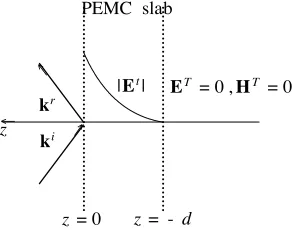
Figure 2. Plane-wave incident on the interface of PEMC slab creates a field transmitted into the slab whose magnitude obeys the function sinh(kx(z+d)). In the regionz <−dthe fields vanish.

To satisfy the interface condition at z = 0 we assume that there exist two plane waves in the PEMC slab denoted by Et+ and Et−. These fields are transverse to the z axis and have the dependence on

x andz

Et(r) = exp(−jkxx)

Et+exp(kxz) +Et−exp(−kxz)

, (93)

Ht(r) = −Mexp(−jkxx)

Et+exp(kxz) +Et−exp(−kxz)

.(94)

Since they vanish atz=−d, we can write

with

Et±=±Etexp(±kxd). (97) Now the interface conditions atz= 0 imply the same reflection as from the PEMC half space. Thus, the condition (42) takes the modified form

Et= E i

t−M ηoJt·Eit (1 + (M ηo)2) sinh(kxd)

, (98)

which inserted in (93) with (97) taken into account yields the total field in the PEMC slab as

Et(r) = 2 exp(−jkxx) sinh(kx(z+d)) (1 + (M ηo)2_{) sinh(k}

xd)

Ei_t−M ηoJt·Eit

. (99)

As two special cases, ford→ ∞the expression (76) for the PEMC half space is reproduced while for the normal incidence casekx →0 of [7], (99) corresponds to the field

Et(r) = 2(z+d) (1 + (M ηo)2)d

Ei_t+M ηouz×Eit

, (100)

which represents linear dependence on thez coordinate.

5. CONCLUSION

In this paper the problem of finding fields reflected from and transmitted through the interface of a PEMC half space or slab has been analyzed. In contrast to an earlier study, obliquely incident time-harmonic plane wave was assumed. Assuming the PEMC conditions (1) it was shown that the field inside the PEMC medium is not unique even if we extract an unphysical metafield component which does not depend on the incident field. However, if the PEMC is defined as a limiting case of a Tellegen medium, with infinitely large parameters, uniqueness can be attained.

ACKNOWLEDGMENT

The authors are thankful for the referee for pointing out the references [10–14].

REFERENCES

2. Lindell, I. V. and A. H. Sihvola, “Transformation method for problems involving perfect electromagnetic conductor (PEMC) structures,” IEEE Trans. Antennas Propagat., Vol. 53, No. 9, 3005–3011, September 2005.

3. Hehl, F.W. and Y. N. Obukhov, Foundations of Classical

Electrodynamics, Birkh¨auser, Boston, 2003.

4. Obukhov, Y. N. and F. W. Hehl, “Measuring piecewise constant axion field in classical electrodynamics,” Phys. Lett., Vol. A341, 357–365, 2005.

5. Lindell, I. V. and A. H. Sihvola, “Losses in the PEMC boundary,”

IEEE Trans. Antennas Propagat., Vol. 54, No. 9, 2553–2558,

September 2006.

6. Lindell, I. V.,Differential Forms in Electromagnetics, Wiley, New York, 2004.

7. Jancewicz, B., “Plane electromagnetic wave in PEMC,”Journal of

Electromagnetic Waves and Applications, Vol. 20, No. 5, 647–659,

Nov. 19, 2006.

8. Kong, J. A., Electromagnetic Wave Theory, 2nd edition, Chap. 3.2, Wiley, New York, 1990.

9. Szekeres, P., A Course in Modern Mathematical Physics, 155, Cambridge University Press, 2004.

10. Lindell, I. V. and A. H. Sihvola, “The PEMC resonator,”Journal

of Electromagnetic Waves and Applications, Vol. 20, No. 7, 849–

859, 2006.

11. Ruppin, R., “Scattering of electromagnetic radiation by a perfect electromagnetic conductor sphere,” Journal of Electromagnetic

Waves and Applications, Vol. 20, No. 12, 1567–1576, 2006.

12. Hussain, A., Q. A. Naqvi, and M. Abbas, “Fractional duality and perfect electromagnetic conductor (PEMC),” Progress In

Electromagnetics Research, PIER 71, 85–94, 2007.

13. Hussain, A. and Q. A. Naqvi, “Perfect electromagnetic conductor (PEMC) and fractional waveguide,”Progress In Electromagnetics

Research, PIER 73, 61–69, 2007.

14. Fiaz, M. A., A. Abdul, A. Ghalfar, and Q. A. Naqvi, “High-frequency expression for the field in the caustic region of a PEMC Gregorian system using Maslov’s method,” Progress In