EDDY CURRENTS IN SOLID RECTANGULAR CORES
S. K. Mukerji, M. George, M. B. Ramamurthy and K. Asaduzzaman
Faculty of Engineering & Technology Multimedia University
Melaka 75450, Malaysia
Abstract—An expression for the eddy current loss in solid rectangular cores is obtained using linear electromagnetic field analysis. Wherefrom text book formula for eddy current loss is derived highlighting various assumptions involved. To get an insight into the current interruption phenomena, electromagnetic fields in a composite rectangular core are analyzed. It is concluded that the reduction in eddy current loss in a laminated cores is basically due to the insertion of distributed capacitors in eddy current paths. Presence of these capacitors increases the impedance of the eddy current path, reducing eddy currents and eddy current loss.
1. INTRODUCTION
Time-varying magnetic fields are established in the core of a coil carrying alternating currents. This may result in eddy currents leading to eddy current loss in the core. Expressions for eddy current loss commonly found in text books [1–3] are derived using lumped circuit approach and assumed eddy current paths. Eddy current loss per unit volume of a thin plate is given by
Pe= π2
6 B
2
mf2T2σ (1)
whereBm,f,T and σ indicate maximum value of flux density, supply
frequency, plate thickness and conductivity respectively.
Since loss density, Pe, is proportional to the square of plate
It is an experimental fact that the eddy current loss in a core with finite cross-section, is reduced if the core is laminated [4, 5]. Fitzgerald et al. [6] observe that magnetic structures are usually built of thin sheet of laminations of the magnetic material. These laminations are insulated from each other. This greatly reduces the magnitude of eddy currents since the layers of insulation “interrupt” the current path. It is often surmised [7–9] that this “interruption” totally blocks eddy currents in one lamination from flowing into the other, thereby altering the shape and size of eddy current paths, thus reducing the eddy current loss.
Many technical papers have been published on electromagnetic transients [10–16] resulting eddy currents. In this paper, using linear electromagnetic field analysis, an expression for the eddy current loss in solid rectangular core subjected to sinusoidal excitation current is found. Wherefrom, based on simplification of the actual conditions, Eq. (1) is developed as a special case,. Also, to glean an insight into the current interruption phenomena, electromagnetic fields in a composite rectangular core are analyzed.
The work reported in the companion paper [17] takes cognizance of the current interruption in laminated cores.
2. HOMOGENEOUS RECTANGULAR CORES
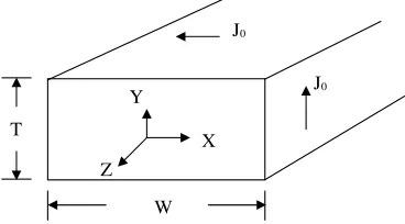
Consider a long magnetic core of width W and thicknessT, as shown in Fig. 1. The exciting coil carrying an alternating current
i=Iejωt (2)
is simulated by a surface current density
Jo =I·N (3)
whereN indicates the number of turns per unit core length.
Y X Z
J
T
0
J0
The current carrying coil will produce a magnetic field Hz. This
time varying field will induce eddy currents in the conducting core. The magnetic field outside the coil is neglected. Maxwell’s equations for harmonic fields are:
∇ ×E = −jωµH (4.1)
∇ ×H = (σ+jωε)E (4.2)
∇ ·E = 0 (4.3)
∇ ·H = 0 (4.4)
Therefore, for constant permeability µ:
∇2H=−γ2H (5)
where
γ =
ω2µε−jωµσ≈(1−j)
ωµσ
2 (6)
This is a two dimensional problem as fields vary along x- and y -directions only. Thus
∂2H z ∂x2 +
∂2H z ∂y2 =−γ
2H
z (7)
The boundary conditions for the magnetic fieldHz, in the core are
Hz=Jo, atx=±W/2, over (−T /2)< y <(T /2) (8.1)
and
Hz=Jo, aty=±T /2, over (−W/2)< x <(W/2) (8.2)
Therefore, the solution for Eq. (7) can be given as follows:
Hz= ∞
p=1 amcos
mπ
W x
· cosh (αmy)
cosh (αmT /2)
+
∞
q=1 bncos
nπ
T y
· cosh (βnx)
cosh (βnW/2)
(9) for (−W/2)< x <(W/2) and (−T /2)< y <(T /2)
where, αm=
mπ
W 2
−γ2 (9.1)
and
βn=
nπ
T 2
m= 2p−1
and
n= 2q−1
while, the Fourier coefficients for rectangular waveforms are:
am =Jo
4
mπsin
mπ
2
(10.1)
and
bn=Jo
4
nπsin nπ
2
(10.2)
The distribution of eddy current density in the homogeneous core can be found using
J =σE (11)
where σ indicates the conductivity of the core material. Therefore in view of Eq. (4.2)
J =δ(∇ ×H) (12)
where,
δ= σ
σ+jωε (12.1)
Thus from Eqs. (9) and (12):
Jx = ∞
p=1
(δαm)amcos
mπ
W x
· sinh (αmy)
cosh (αmT /2)
−∞
q=1
δnπ T
bnsin
nπ
T y
· cosh (βnx)
cosh (βnW/2)
(13)
Jy = ∞
p=1
δmπ W
amsin
mπ
W x
· cosh (αmy)
cosh (αmT /2)
−∞
q=1
(δβn)bncos
nπ T y
· sinh (βnx)
cosh (βnW/2)
(14)
Next, consider the complex Poynting vector and its components, as given below,
P = 1 2E×H
∗ (15)
Px=
1 2σJyH
∗
and
Py =−
1 2σJxH
∗
z (15.2)
Now, eddy current loss per unit core length,Peis given as the real part
of Pc, the complex power per unit core length. While
Pc =−2 T /2
−T /2
Px|x=W/2dy−2 W/2
−W/2
Py|y=T /2dx (16)
Using Eqs. (10.1), (10.2), (13) and (14), one gets in view of Eqs. (6), (9.1), (9.2) and, (12.1):
Pc=
8
π2JoJ ∗ ojωµ W ∞ p=1
tanh (αmT /2) m2α
m
+T ∞
q=1
tanh (βnW/2) n2β
n (17)
where, m= 2p−1andn= 2q−1.
Therefore the loss density Pe, in the rectangular core is given by:
Pe=
8
π2JoJo∗ωµ W ∞ p=1
αmisinh (αmrT)−αmrsin (αmiT) m2α2
mr+α2mi
[cosh (αmrT) + cos (αmiT)]
+T ∞
q=1
βnisinh (βnrW)−βnrsin (βniW) n2β2
nr+βni2
[cosh (βnrW) + cos (βniW)] (18) where,
αmr=Re [αm]
=√1 2 mπ W 2
−ω2µε 2
+ω2µ2σ2+
mπ
W 2
−ω2µε 1 2 (18.1)
αmi=Im [αm]
=√1 2 mπ W 2
−ω2µε 2
+ω2µ2σ2−
mπ
W 2
−ω2µε 1 2 (18.2)
βnr=Re [βn]
=√1 2 nπ T 2
−ω2µε 2
+ω2µ2σ2+
nπ
T 2
βni=Im [βn]
=√1 2
nπ
T 2
−ω2µε 2
+ω2µ2σ2−
nπ
T 2
−ω2µε
1 2
(18.4)
The expression for eddy current loss per unit core length given in Eq. (18) is quite involved. This can, however, be simplified by noting that the hyperbolic functions are usually much larger than sinusoidal functions. Thus for large values of (αmr·T) and (βnr·W), on setting
tan hyperbolic functions to unity:
Pe≈
8
π2JoJo∗jωµ W
∞
p=1
αmi m2α2
mr+α2mi +T
∞
q=1
βni n2β2
nr+βni2
(19)
where, m= 2p−1 and n= 2q−1.
A further simplification is possible if both (π/W) and (π/T) are large compared to√ωµσ. Therefore for small values of σ, in view of Eqs. (18.1)–(18.4), Eq. (19) reduces to:
Pe≈
4
π5SJoJo∗ω
2µ2σW4+T4 (20)
where,
S =
∞
p=1
1
m5 (20.1)
where, m= 2p−1.
The value ofS found from tables [18, 19] is
S = 1.00452≈1 (20.2)
Alternatively for large values of σ, only the first terms in the two fast converging infinite series involved in Eq. (19) could be retained. Then, from Eqs. (9.1) and (9.2):
α1≈β1 ≈jγ (21)
Thus, using Eq. (6)
α1 ≈β1 ≈(1 +j)
ωµσ
Therefore from Eq. (19), for large values ofσ
Pe ≈
4√2
π2 JoJo∗
ωµ
σ [W +T] (23)
A large conducting plate of thickness T, can be considered as a special case of the rectangular core with its width, W, tending to infinity. While, the eddy current loss per unit plate volume, pe, is
given by
pe= (Pe/W T)|w→∞ (24)
Therefore, in view of Eqs. (9.1), (6), (18) and (24), one gets:
pe≈JoJo∗
ωµ
2σ T1
sinh
ωµσ
2 ·T
−sin
ωµσ
2 ·T
cosh
ωµσ
2 T
+ cos
ωµσ
2 T
(25)
Therefore, for thick plates
pe≈JoJo∗
ωµ
2σ 1
T
(25.1)
while for thin plates,
pe≈JoJo∗ σ
24ω
2µ2T2 (25.2)
This leads to Eq. (1), on substituting 2πf forω and B2
m forµ2JoJo∗.
3. COMPOSITE MAGNETIC CORES
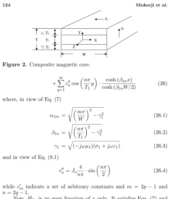
Let the homogeneous core in Fig. 1 be replaced by a composite core, made up of two different materials and placed symmetrically inside the current carrying coil, as shown in Fig. 2.
Three core-regions can be identified, viz, region-1 (or central region) for (−T1/2)< y <(T1/2); region-2 (or top region) for (T1/2)< y <(T /2) and region-3 (or bottom region) for (−T /2)< y <(−T1/2).
Each region extends over (−W/2)< x <(W/2). In view of symmetry it will be sufficient to consider, say, the first two regions. We shall use suffix-1, to indicate region 1 and suffix-2, to indicate region-2.
Noting thatH1z is an even function ofxandy; further, it satisfies
Eqs. (7) and (8.1). Let
H1z = ∞
p=1 cmcos
mπ
W x
· cosh (α1my)
Y
X
Z
J0
J0
T2
T
T2
T1
W
1/2
1/2
Figure 2. Composite magnetic core.
+
∞
q=1 cncos
nπ T1 y
· cosh (β1nx)
cosh (β1nW/2)
(26)
where, in view of Eq. (7)
α1m =
mπ
W 2
−γ2
1 (26.1)
β1n =
nπ T1
2
−γ12 (26.2)
γ1 =
(−jωµ1)(σ1+jωε1) (26.3)
and in view of Eq. (8.1)
cn=Jo
4
nπ ·sin
nπ
2
(26.4)
while cm indicate a set of arbitrary constants and m = 2p−1 and
n= 2q−1.
Now, H2z is an even function ofx only. It satisfies Eqs. (7) and
(8.1). Further,
H2z =H1z, aty=T1/2 over (−W/2)< x <(W/2) (27.1)
and
H2z=Jo, aty=T /2 over (−W/2)< x <(W/2) (27.2)
Therefore,
H2z = ∞
p=1
cos
mπ
W x
dm
sinhα2m(y−T1/2)
sinh(α2mT2/2) −
cmsinhα2m(y−T /2)
+
∞
q=1
cncosn2π
T2
y−T1
2 −
T2
4
· cosh (β2nx)
cosh (β2nW/2)
(28)
where, in view of Eq. (7),
α2m =
mπ
W 2
−γ2
2 (28.1)
β2n =
n2π T2
2
−γ22 (28.2)
γ2 =
(−jωµ2) (σ2+jωε2) (28.3)
and in view of Eq. (27.2)
dm =Jo
4
mπsin
mπ
2
(28.4)
and m= 2p−1, n= 2q−1.
To find the arbitrary constant cm, consider the distribution of electric field in the two regions. In view of Eqs. (12), (12.1), (26) and (28), the distribution of eddy current density in region-1 is obtained as:
J1x = ∞
p=1
(δ1α1m)cmcos
mπx W
sinh (α1my)
cosh
α1m
T1
2
−∞
q=1
δ1 nπ
T1
cnsin
nπy
T1
cosh (β1nx)
cosh
β1n
W
2
(29.1)
and
J1y = ∞
p=1
δ1 mπ
W
cmsin
mπx
W
cosh (α 1my)
cosh
α1m
T1
2
−∞
q=1
(δ1β1n)cncos
nπy T1
sinh (β1nx)
cosh
β1n
W
2
(29.2)
where, m= 2p−1, n= 2q−1 and
δ1=
σ1
(σ1+jωε1)
and in region-2, as:
J2x= ∞
p=1
(δ2α2m) cos mπx W × dm
coshα2m
y−T1
2 sinh α2m T2 2
−cm
coshα2m
y−T
2 sinh α2m T2 2 −∞ q=1 δ2 n2π
T2
cnsinn2π
T2
y−T1
2 −
T2
4
cosh (β2nx)
cosh β2n W 2 (30.1) and
J2y = ∞ p=1 δ2 mπ W sin mπx W × dm
sinhα2m
y−T1
2 sinh α2m T2 2
−cm
sinhα2m
y−T
2 sinh α2m T2 2 −∞ q=1
(δ2β2n)cncos n2π
T2
y−T1
2 −
T2
4
sinh (β 2nx)
cosh β2n W 2 (30.2)
where, m= 2p−1, n= 2q−1 and
δ2=
σ2
(σ2+jωε2)
(30.3)
Now, since,
J1x σ1
= J2x
σ2
, aty=T1/2, over (−W/2) < x <(W/2) (31)
Eqs. (29.1) and (30.1) give,
∞ p=1 δ1 σ1 α1m
tanh (α1mT1/2)cmcos mπ W x −∞ q=1 δ1 σ1 nπ T1
sin (nπ/2)cn cosh (β1nx)
= ∞ p=1 δ2 σ2 α2m
dmcosech (α2mT2/2)−cmcoth(α2mT2/2) cos mπ W x + ∞ q=1 δ2 σ2
n2π T2
sin (nπ/2)cn cosh (β2nx)
cosh (β2nW/2)
over (−W/2)< x <(W/2) (32)
and where, m= 2p−1, n= 2q−1.
Considering the Fourier series expansion:
cosh (βnx)
cosh (βnW/2)
= ∞ p=1 4 W mπ W sin mπ 2 mπ W 2
+βn2 cos mπ W x (33)
over (−W/2)< x <(W/2) and where, m= 2p−1. We get from Eq. (32)
δ1 σ1
α1m
tanh (α1mT1/2)+
δ2 σ2
α2m
coth (α2mT2/2)
cm
= δ2 σ2 α2m
cosec (α2mT2/2)dm+
4 W mπ W sin mπ 2 δ1 σ1 1 T1 ∞ q=1 nπsin nπ 2 β2 1n+ mπ W
2cn+ δ2 σ2 2 T2 ∞ q=1 nπsin nπ 2 β2 2n+ mπ W 2 cn
(34)
where, n= 2q−1.
Now, in view of Eqs. (26.1), (26.2) and (26.4)
∞ q=1 nπsin nπ 2
β1n2 +
mπ
W
2cn= ∞
n−odd
4Jo(T1/π)2
n2+
T1 π α1m
2 (34.1)
where, n= 2q−1 and in view of Eqs. (28.1), (28.2) and (26.4)
∞ q=1 nπsin nπ 2
β22n+
mπ
W
2cn= ∞
q=1
4Jo(T2/2π)2
n2+
T2
2πα2m
where, n= 2q−1.
These infinite series can be summed up [11, 12]. Thus, using the identity:
∞
q=1
1
n2+θ2 ≡ π
4θtanh
π
2θ
(35)
where,n= 2q−1 and Eqs. (34) and (28.4), the expression forcmfound as:
cm =
4
WJosin
mπ
2
δ1 σ1
mπ/W
α1m
tanh (α1mT1/2)
+ 4
WJosin
mπ
2
δ2 σ2
mπ/W
α2m
tanh (α2mT2/4)
+ α2m
mπ/Wcosech (α2mT2/2)
δ1 σ1
α1m
tanh (α1mT1/2) +
δ2 σ2
α2m
coth (α2mT2/2) (36)
4. DISCUSSION
Expressions for eddy current loss in the solid rectangular core are given by eqns. (18), (19), (20) and (23). From each of these equations it can be concluded that for a given core area and coil current, the loss density is minimum for a core with square cross section. Incidentally, for each metre of coil length, both the amount of copper in the coil as well as the copper loss will also be minimum in the case of a square cross section.
For the rectangular core, the eddy current density,Jy, is given by
eqn. (14). This component of eddy current density vanishes as the core width, W, tends to infinity. Therefore, in large plates, eddy currents flow parallel to the plate surfaces. Thus if the plate is laminated, eddy currents are not interrupted. However, because of non-zero thickness of interlaminar insulation, laminating large plates alters the distribution of eddy currents in the plate volume.
Consider the composite core shown in Fig. 2. It may be seen from Eqs. (29.2) and (30.2), that the normal component of both, the displacement- and the conduction-current densities are continuous at the boundary between the two adjacent regions, provided that the relaxation times for these regions are identical.
T2
T1 T
T2 INSULATION
INSULATION
+ + +
-+ -+ -+
W
T2
T1 T
T2 +
-+
W
---Eddy currents Displacement currents (Figure not to scale)
(a) (b)
1/2
1/2
1/2
1/2
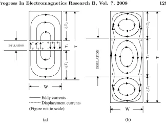
Figure 3. Cross-sectional view of composite cores with perfect insulation. (a) Small insulation thickness, (b) Large insulation thickness.
In view of eqns. (29.1), (29.2) and (29.3), there will be no eddy currents in region-1 when the conductivity of this region, s1, is zero. Eddy currents in region-2 and -3, flowing in open paths deposit charges on the two interfaces between conducting and non-conducting regions, vide Fig. 3. The region-1 provides a distributed capacitance in the eddy current paths. For a non-zero conductivity of region-1, σ1, eddy
currents flow through leaky capacitance. It is therefore, concluded that even with perfect interlaminar insulation, eddy currents in a lamination are not totally restrained from flowing into another.
5. CONCLUSION
The presence of capacitance in the eddy current path increases the impedance of the path. Thus reducing eddy currents and eddy current loss for a given core flux.
REFERENCES
1. Golding, E. W., Electrical Measurements and Measuring
Instru-ments, 4th edition, 521–528, Sir Isaac Pitman & Sons, Ltd.,
Lon-don, 1955.
2. Langsdorf, A. S., Theory of Alternating Current Machinery, 2nd edition, 34–36, Tata McGraw-Hill Publishing Co. Ltd., 1999. 3. Gupta, J. B.,Theory&Performance of Electrical Machines, 13th
edition, Part-III, 32–34, S. K. Kataria & Sons, 2000.
4. Say, M. G., Performance and Design of Alternating Current
Machines, 3rd edition (first Indian edition), 175–176, CBS
Publishers & Distributors, 1983.
5. Reed, M., “An experimental investigation of the theory of eddy currents in laminated cores of rectangular section,” Jour. IEE, Vol. 80, 567.
6. Fitzgerald, A. E., C. Kingsley, Jr., and S. D. Umans, Electric
Machinery, 6th edition, 26, McGraw-Hill, 2003.
7. Stephen, J. C., Electric Machinery Fundamentals, WCB/3rd edition, 30, McGraw-Hill, 1999.
8. Charles, I. H., Electric Machines
(Theory,Operation,Applica-tions,Adjustment,and Control), 2nd edition, 28, Pearson
Educa-tion, Inc., Prentice Hall, 2002.
9. Theodore, W., Electrical Machines,Drives,and Power Systems, 5th edition, 35, Pearson Education, New Jersy, 2002.
10. Poljak, D. and V. Doric, “Wire antenna model for transient analysis of simple grounding systems, Part I: The vertical grounding electrode,” Progress In Electromagnetics Research, PIER 64, 149–166, 2006.
11. Poljak, D. and V. Doric, “Wire antenna model for transient analysis of simple grounding systems, Part II: The horizontal grounding electrode,” Progress In Electromagnetics Research, PIER 64, 167–189, 2006.
12. Tang, M. and J. F. Mao, “Transient analysis of lossy nonuniform transmission lines using a time-step integration method,”Progress
In Electromagnetics Research, PIER 69, 257–266, 2007.
13. Fau, Z., L. X. Ran, and J. A. Kong, “Source pulse optimization for UWB radio systems,”Journal of Electromagnetics Waves and
Applications, Vol. 20, No. 11, 1535–1550, 2006.
Vol. 20, No. 12, 1681–1694, 2006.
15. Mukerji, S. K., G. K. Singh, S. K. Goel, and S. Manuja, “A theoretical study of electromagnetic transients in a large conducting plate due to current impact excitation,” Progress In
Electromagnetics Research, PIER 76, 15–29, 2007.
16. Mukerji, S. K., G. K. Singh, S. K. Goel, and S. Manuja, “A theoretical study of electromagnetic transients in a large plate due to voltage impact excitation,” Progress In Electromagnetics
Research, PIER 78, 377–392, 2008.
17. Mukerji, S. K., M. George, M. B. Ramamurthy, and K. Asaduzza-man, “Eddy currents in laminated rectangular cores,” a compan-ion paper.
18. Jolley, L. B. W., Summation of Series, 2nd revised edition, 240, Dover Publications, Inc., 1961.
19. Philip, M. M. and H. Fishbach, Methods of Theoretical Physics, Part-I, 413–414, McGraw-Hill Book Company, Inc. and Ko Gakusha Company, Ltd., 1953.
20. Chen, H., B. I. Wu, and J. A. Kong, “Review of electromagnetic waves in left-handed materials,” Journal of Electromagnetics
Waves and Applications, Vol. 20, No. 15, 2137–2151, 2006.
21. Grzegorczyk, T. M. and J. A. Kong, “Review of left-handed materials: Evolution from theoretical and numerical studies to potential applications,” Journal of Electromagnetics Waves and
Applications, Vol. 20, No. 14, 2053–2064, 2006.
22. Mahmoud, S. F. and A. J. Viitanen, “Surface wave character on a slab of metamaterial with negative permittivity and permeability,”