Available online: https://edupediapublications.org/journals/index.php/IJR/ P a g e | 2823
A New Methodology for Identifying Node Issues in Network
Topologies
KAKARLA SRILEKHA , PG student,Dept of MCA, Rajeev Gandhi Memorial College of Engineering
and Technology,
S.Parimala, Assistant professor,Dept of MCA, Rajeev Gandhi Memorial College of Engineering
and Technology,
C.Lakshmi, Assistant professor, Dept of MCA, Rajeev Gandhi Memorial College of Engineering
and Technology.
ABSTRACT
Recognizing the event and area of execution
investigation is hard to ensuring the viable
activity of framework foundations. In this paper
we present a structure for identifying and
restricting execution inconsistencies in light of
using a dynamic test engaged estimation system
conveyed on the outskirts of a system
association. Boolean framework tomography is a
compelling instrument to construe the state
(working/crossed out) of individual center points
from way level estimations removed by
edge-centers. We consider the issue of enhancing the
capacity of perceiving framework
disappointments through the usage of observing
techniques. Finding a perfect arrangement is
NP-hard and an extensive gathering of work has
been given to heuristic procedures giving lower
limits. Not at all like past works, we give upper
limits on the most elevated number of
identifiable center points, given the quantity of
observing ways and different requirements on
the framework topology, the directing approach,
additionally, the most elevated way length. The
proposed upper limits depicts to a noteworthy
point of confinement on the identifiability of
disappointments by methods for Boolean
framework tomography. This examination gives
encounters on the most capable technique to
plan topologies and related observing plans to
accomplish the most elevated identifiability
under various system settings. Through
examination and tests we demonstrate the
snugness of the limits and suitability of the
outline bits of knowledge of information for
designed and authentic systems.
Keywords: Network Tomography; Node Failure Localization; Identifiability Condition;
Maximum Identifiability
I. INTRODUCTION
The capability to evaluate the conditions
of network nodes in the presence of node
failures is key for some functions in network
system management, including performance
investigation, route decision, and system
recovery. In present day networks, the modern
Available online: https://edupediapublications.org/journals/index.php/IJR/ P a g e | 2824 node failures is not any more sufficient, as bugs
and setup errors in different client programming
and system functions frequently induce
"noiseless failures" that are just noticeable from
end to-end connection states. Boolean system
tomography is an effective tool to surmise the
conditions of individual hubs of a network from
binary measurements brought along selected
paths. One such approach, for the most part
known as network tomography, concentrates on
inducing inside network characterstics in view
of end-to-end performance calculations from a
subset of hubs with observing capabilities, called
to as monitors. Dissimilar to straight
measurement, network tomography just depends
on end-to-end performance experienced by
information packets, in this path tending to
issues such as overhead, lack of convention
support, and noiseless failures. In situations
where the system characteristics for interest is
binary (e.g., typical or failure), this approach is
known as Boolean network tomography. In this
paper, we think about a utilization of Boolean
network tomography to localize hub failures
from calculations of path states. Under the
suspicion that a measurement path is ordinary if
and just if all hubs on this path carry on
regularly, we detail the issue as a system of
Boolean conditions, where the unknown factors
are the binary hub states, and the known
constants are the observed conditions of
measurement paths. The objective of Boolean
network tomography is basically to settle this
network of Boolean equations. Since the
perceptions are coarse-grained (path
ordinary/failed), it is generally difficult to
exceptionally distinguish node states from path
measurements. For instance, if two hubs
continuously seem together in measurement
paths, at that point upon observing failures of
every one of these paths, we can at generally
find that one of these hubs (or both) has failed
yet can't decide which one. Since there are
frequently various explanations for given path
failures, existing work for the most part
concentrates on finding the minimum
arrangement of failed nodes that most likely
includes failed nodes. Such an approach, in any
case, does not ensure that hubs in this minimum
set have failure or that hubs outside the set have
not. By and large, to recognize two achievable
failure sets, there must exist an estimation path
that crosses one and just a single of these two
sets. To decide such one of kind failure
localization in sub-systems, we have to see how
it is identified with network properties. We will
think about every one of these issues with
regards to the accompanying classes of probing
methods: (a) Controllable Arbitrary-path
Probing (CAP), where any measurement path
can be set up by monitors, (b) Controllable
Straightforward path Probing (CSP), where any
measurement path can be set up, if it is cycle
Available online: https://edupediapublications.org/journals/index.php/IJR/ P a g e | 2825 measurement paths are dictated by the default
routing protocol.
II. PROBLUM DEFINATION
We use lower-case letters to denote scalars and
vectors and upper-case letters to denote
matrices. For a vector p, p|i denotes the i-th
element in the vector. For a matrix M, M|i,j
denotes the element in the i-th row and j-th
column; moreover, M|i,∗ denotes the i-th row
and M|∗,j the j-th column of M.
Network Setup Model
We describe the network as an undirected chart
G = (V, E), where V is a number of n nodes, and
E is the number of connections. Every node
might be in ordinary or failure state. Without
loss of all inclusive statement, we accept that
connections don't fail, as connection failures can
be designed by the failures of consistent nodes
that speak to the connections. The arrangement
of all failures nodes, meant by F ⊆ V,
characterizes the state of a system, and is called
failure set.
Perception Model
We expect that node states can't be estimated
straightforwardly, in any case, just in a
roundabout way by means of monitoring paths.
Let P = {p1, p2. . . pm} be a given number of m
monitoring paths. According to the requirements
of the decision, every path pi ∈ P is describes to
as either an collection of nodes pi, or as a
requested grouping of hubs pˆi, from one
endpoint to the next. The state of a path is
typical if and just if all crossed nodes are in
ordinary state. We call the incident set of vi the
arrangement of ways influenced by the failure of
hub vi and signify it with Pvi. We likewise
indicate the occurrence set of paths of a failure
set F with PF, ∪vi∈F Pvi. The testing
framework T is a m × n grid, where T|i,j = 1 on
the off chance that vj ∈ pi , and zero generally.
The j-th segment of T, indicated with b(vj ) ,
T|∗,j , is the trademark vector1 of Pvj . The
transpose of b(vj ) is thusly called the binary
encoding of vj . Note that numerous hubs may
have a similar binary encoding.
Identifiability
The idea of identifiability describes to the
capability of deriving the states of individual
hubs from the states of the monitoring paths.
Casually, we say that a hub v is 1-identifiable,
given a number of paths P, if its failure and the
failure of some other hub w cause the failure of
various sets of monitoring paths in P, i.e. v and
w have distinctive episode sets. This idea can be
extended out to the instance of simultaneous
failures of at most k nodes, where a hub is
k-identifiable in P if any two set of failures F1 and
F2 of size k, which contrast at any rate in v (i.e.,
Available online: https://edupediapublications.org/journals/index.php/IJR/ P a g e | 2826 failures of various monitoring paths in P, i.e. F1
and F2 have various difference incident sets.
Bounding Identifiability
The number of monitoring paths P is typically
the outcome of outline choices identified with
topology, observing endpoints, routing scheme,
and so forth. Given a set of candidate path sets P
under every possible outline, the query is: the
manner by which well would we be able to
monitor system utilizing path measurements and
which configuration is the best? Utilizing the
idea of k-identifiability, we can quantify the
monitoring performance by the set of nodes that
are k-identifiable with respect to P, indicated by
φk(P), and define this query as an advancement: ψk(P) , maxP ∈P φk(P). Although broadly
considered, the ideal solution is difficult to get
due to the (exponentially) substantial size of P,
and heuristics are utilized to give lower bounds.
There is, nonetheless, an absence of general
upper bounds. In this work we set up upper
bounds on ψk(P) in representive situations.
Learning of these upper bounds is vital to
comprehension the basic limits of Boolean
network tomography, and gives bits of
knowledge on network configuration to
encourage network monitoring.
III. IMPACT OF PROBING MECHANISMS
Based upon the adaptability of probing
furthermore, the cost of deployment, we
categorize probing components into one of three
classes: A) Controllable Arbitrary path Probing
(CAP): P incorporates any path/cycle, permitting
repeated hubs/links, gave every path/cycle
begins and finishes at (the same or unique)
screens. 2) Controllable Simple path Probing
(CSP): P incorporates any basic (i.e., free cycle)
path between various screens. 3) Uncontrollable
Probing (UP): P is the collection of paths
between screens described by the routing
protocol utilized by the system, not controllable
by the screens. In spite of the fact that CAP
enables probes to navigate every hub/connection
and subjective number of times, it does the trick
to consider paths where each probe navigates
each connection at most once in either course for
localizing hub failures.
Fig1. Sample network with three monitors: m1, m2, and
m3.
Alternatively, CSP can be designed by
deploying Virtual Private Networks over IP
systems, where the free cycle property is
likewise required while choosing paths between
VPN end points. These examining systems
plainly give diminishing adaptability to the
screens and subsequently diminishing capacity
to restrict failures. Notwithstanding, they
Available online: https://edupediapublications.org/journals/index.php/IJR/ P a g e | 2827 organization. Top speaks to the most adaptable
monitoring system and gives an upper bound on
disappointment restriction capacity. In
customary systems, CAP is doable at the IP
layer if strict source routing is empowered at all
nodes,3 or at the application layer if proportional
"source steering" is bolstered by the application.
Additionally, CAP is likewise practical under a
rising systems administration worldview called
programming characterized organizing (SDN),
where screens can train the SDN controller to set
up subjective ways for the probing traffic.
conversely, UP speaks to the most fundamental
probe mechanism, achievable in any
correspondence arrange, that gives a lower
bound on the capacity of failures limitation
Alternatively, CSP can be actualized by sending
Virtual Private Networks over IP systems, where
the sans cycle property is additionally required
while choosing ways between VPN
end-focuses. These three probing components
extracted the principle features of a few existing
and developing routing methods. Our objective
is to measure how the adaptability of a probe
component influences the system's capacity to
localize failures.
IV. VERIFIABLE IDENTIFIABILITY
CONDITIONS
Given the above outcomes, we are currently
prepared to measure the effect of the probe
mechanisms on hub failure localization. We
intend to measure this effect by evaluating,
utilizing our bounds on the most extreme
identifiability, the number of concurrent failures
we can particularly localize in a given system
with a given screen placement under each of the
three probing mechanisms (CAP, CSP, UP). In
this investigation, we expect (hop count based)
shortest path routing as the default directing
protocol under UP, i.e., the measurement paths
under UP are the shortest paths between screens,
with ties broken arbitrarily.
Fig 2: Enhanced Random Monitor Placement (ERMP)
Given a system topology G, a set of screens M,
and a probing mechanisms (CAP, CSP, or UP),
we try to reply the following firmly related
questions: (I) Given a hub set of interest S and a
bound k on the quantity of failures, can we
extraordinarily localize up to k failed hubs in S
Available online: https://edupediapublications.org/journals/index.php/IJR/ P a g e | 2828 S, what is the greatest number of failures inside
S that can be exceptionally localized? (iii)
Given a whole number k (1 ≤ k ≤ σ), what is the
biggest node set that is k-identifiable? We will
analyze these issues from the viewpoints of the
two theories and proficient algorithms.
V. PERFORMANCE EVALUATION
We concentrate on evaluating per-hub most
extreme identifiability index Ω (v) since it
decides both the per-set highest identifiability
index Ω (S) and the most extreme identifiable
set S* (k). Specifically, the complementary
cumulative distribution function (CCDF) of Ω
(v) over all v ∈ N coincides with the
standardized cardinality of the greatest
identifiable set |S* (k)|/σ, and along these lines
we describe the dispersion of Ω (v) by assessing
|S* (k)|/σ with respect to k. Also, we inspect the
particular value of Ω (v) and compare it and the
degree (i.e., number of neighbors) of v among
screen/non-screen nodes to assess the connection
between the greatest identifiability index and the
graph theoretic property (i.e., degree) of a node.
At the point when the correct values of Ω (v)
and |S* (k)| can't be evaluated (under CSP also,
UP), we evaluate the upper/bring down bounds
and plot the zone between the bounds. Under
UP, our broad simulations under numerous
graph models have demonstrated that MSC (v)
can be nearly approximated by GSC (v); thus,
we utilize GSC (v) set up of MSC (v) for
processing ΩUP and S* UP.
Distribution of Ω (v): To describe the general distribution of Ω (v), we process (bounds on)
𝑆𝐶𝐴𝑃∗ (k), 𝑆𝐶𝑆𝑃∗ (k), what’s more, 𝑆𝑈𝑃∗ (k) to
assess |S* (k)|/σ for various values of k (σ: add
up to number of non-screens). Fig. 4 reports
midpoints of |S* (k)|/σ registered on ER
diagrams over various randomly generated
examples of topology and screen areas, where
|S* (k)|/σ under CSP and UP is spoken to by a
band with its width controlled by (|Souter (k)
|−|Sinner (k)|)/σ. The outcomes indicate
substantial differences in the failure limitation
abilities of various probing mechanisms: When
the set of screens is little (μ = 2) and k = 2, 𝑆𝑈𝑃∗
(k) is relatively unfilled, i.e., no (non-screen)
hub state can be particularly controlled by UP
when there are various failures; conversely,
|𝑆𝐶𝑆𝑃∗ (k)|/σ ≈ 0.5 and |𝑆
𝐶𝐴𝑃∗ (k)|/σ ≈ 1, i.e., CSP
can exceptionally describe the states of half of
the hubs and CAP can decide the states of the
considerable number of nodes when μ = 2 and k
= 2. At the point when the quantity of screens
increments (μ = 10), there exist greater
measurement paths amongst screens, and along
these lines the portion of identifiable nodes
increments for every one of the three examining
mechanisms. Moreover, we watch a steady stage
Available online: https://edupediapublications.org/journals/index.php/IJR/ P a g e | 2829
Fig. 3. Maximum k-identifiable set S* (k) under CAP, CSP, and UP for ER graphs (|V | = 20, μ = {2, 10}, E [|L|] = 51, 200 graph instances, σ: total number of non-monitors). (a) μ = 2. (b) μ = 10
Where the estimation of |S* (k)|/σ continues as
before as we increment k; this is on account of
some non-screens have screens as neighbors, in
this manner straightforwardly quantifiable by
these neighboring screens without navigating
other non-screens. In particular, on the off
chance that there are non-screens that neighbor
no less than one screen under CAP, neighbor no
less than two screens under CSP, or lie on 2 hop
paths between screens under UP, at that point
the failure of these non-screens can simply be
distinguished in any case of the aggregate
number of failures in the system, i.e., the
greatest identifiability index of these
non-screens is the add up to number of non-non-screens.
Note that in Fig. 3,
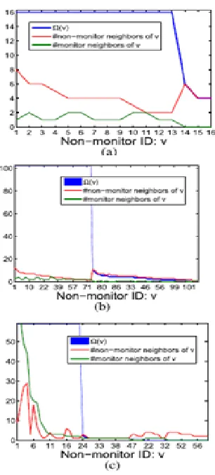
Correlation of Ω (v) and Degree: Next, we
analyze particular values of Ω (v) for each
non-screen v ∈ N for chosen instance of system
topology and screen placement, where Theorems
25 and 26 are utilized for processing the
lower/upper bounds under CSP and UP, framing
a band in Fig.4. We will likely compare these
qualities and hub degrees to understand the
correlation between's the proposed identifiability
measure and graph diagram theoretic hub
properties.
Fig. 4. Node maximum identifiability index Ω (v) of (a) ER graph/ (b) Rocket fuel AS1755/(c) CAIDA under different probing mechanisms
In particular, we sort non-screens in a non
increasing request of Ω(v) under each of the
three probing mechanisms, also, think about
Ω(v) with the degrees of v among
screens/non-screens; get brings about Fig. 4 (b) for irregular
topologies and in Fig.4 (c) for AS topologies.
Available online: https://edupediapublications.org/journals/index.php/IJR/ P a g e | 2830 amongst Ω (v) and the degree of v, meant by
d(v). In particular, signify the quantity of
neighbors of v that are screens by 𝑑𝑚(v) and the
quantity of neighbors of v that are non-screens
by 𝑑𝑛 (v); the general degree d (v) = 𝑑𝑚 (v) +
𝑑𝑛 (v). On the off chance that hub v has
adequate screen neighbors (𝑑𝑚 (v) ≥ 1 for CAP,
𝑑𝑚 (v) ≥ 2 for CSP), at that point v is
specifically measurable what's more, hence
Ω(v) = σ paying little mind to the genuine level
of v; if hub v does not have an adequate number
of screens as neighbors, at that point Ω(v) ≤d(v)
in light of the fact that if all neighbors of v
bomb, at that point the state of v can't be
determined by path measurements. Our
perception likewise focuses on the significance
of enhanced screen placement, particularly when
we are just intrigued by checking a subset of
hubs, which is left to future work.
VI. CONCLUSION
We consider the issue of increasing number of
nodes whose states can be distinguished by
means of Boolean network tomography. We
define the issue as far as graph diagram based
group testing and endeavor the combinatorial
structure of the testing matrix to determine
upper bounds on the set of identifiable hubs
under various presumptions, including:
subjective routing, steady routing, monitoring
through client and server paths with one or
different servers (and even or uneven
distribution of customers), and half-predictable
routing. These bounds demonstrate the central
furthest reaches of Boolean network tomography
in both genuine and engineered systems. Other
than the hypothetical value of this investigation,
we utilize the bounds to determine bits of
insights for the outline of topologies and
monitoring plans with high identifiability in
various system situations. Through examination
also, experiments we assess the tightness of the
bounds and describes the efficiency of the plan
insights of knowledge for engineered and also
genuine systems.
VII. REFERENCES
[1] P. Barford, J. Kline, D. Plonka, and A. Ron,
“A Signal Analysis of Network Traffic
Anomalies,” in Proceedings of ACM
SIGCOMM Internet Measurement Workshop,
November 2002.
[2] A. Lakhina, M. Crovella, and C. Diot,
“Diagnosing Network-wide Traffic Anomalies,” in Proceedings of ACM SIGCOMM ’04, August
2004.
[3] A. Hussain, J. Heidemann, and C.
Papadopoulos, “A Framework for Classifying Denial of Service Attacks,” in Proceedings of ACM SIGCOMM ’03, August 2003.
Available online: https://edupediapublications.org/journals/index.php/IJR/ P a g e | 2831
[5]“Cisco IOS IP SLAs,”
http://www.cisco.com/go/ipsla, 2009.
[6] Y. Bejerano and R. Rastogi, “Robust
Monitoring of Link Delays and Faults in IP
Networks,” in Proceedings of IEEE INFOCOM ’03, April 2003.
[7] A. Dhamdhere, R. Teixeira, C. Dovrolis, and
C. Diot, “NetDiagnoser: Troubleshooting
network unreachabilities using end-to-end
probes and routing data,” in Proceedings of ACM CoNEXT ’07, December 2007.
[8] N. Spring, R. Mahajan, and D. Wetherall,
“Measuring ISP Topologies with Rocketfuel,” in Proceedings of ACM SIGCOMM ’02, August
2002.
[9] H. Zeng, P. Kazemian, G. Varghese, and N.
McKeown, “Automatic test packet generation,”
in ACM CoNEXT, 2012.
[10] H. Nguyen and P. Thiran, “The boolean
solution to the congested IP link location
problem: Theory and practice,” in IEEE
INFOCOM, 2007.
[11] A. Dhamdhere, R. Teixeira, C. Dovrolis,
and C. Diot, “Netdiagnoser: Troubleshooting
network unreachabilities using end-to-end
probes and routing data,” in ACM CoNEXT,