Recursive Least Squares Dictionary Learning Algorithm
for Electrical Impedance Tomography
Xiuyan Li, Jingwan Zhang, Jianming Wang*, Qi Wang, and Xiaojie Duan
Abstract—Electrical impedance tomography (EIT) is a technique for reconstructing conductivity distribution by injecting currents at the boundary of a subject and measuring the resulting changes in voltage. Sparse reconstruction can effectively reduce the noise and artifacts of reconstructed images and maintain edge information. The effective selection of sparse dictionary is the key to accurate sparse reconstruction. The EIT image can be efficiently reconstructed with adaptive dictionary learning, which is an iterative reconstruction algorithm by alternating the process of image reconstruction and dictionary learning. However, image accuracy and convergence rate depend on the initial dictionary, which was not given full consideration in previous studies. This leads to the low accuracy of image reconstruction model. In this paper, Recursive Least Squares Dictionary Learning Algorithm (RLS-DLA) is used to learn the initial dictionary for dictionary learning of sparse EIT reconstruction. Both simulated and experimental results indicate that the improved dictionary learning method not only improves the quality of reconstruction but also accelerates the convergence.
1. INTRODUCTION
EIT is an imaging modality that aims at estimating conductivity distribution within a domain through several electrodes attached to its surface [1]. Pairs of electrodes are consecutively used to generate different current density distributions within the domain. The electric potential of the surface is measured by the other electrodes apart from the current excitation. The cross-sectional conductivity images are reconstructed eventually through the measured potentials.
Due to the serious nonlinearity and ill-posedness of EIT inverse problem, a set of boundary measurements can often obtain lead to solutions that satisfy the condition [2]. Research on reconstruction algorithms is devoted to how to get the optimal solution. In recent years, many reconstruction algorithms have been proposed, such as Tikhonov regularization, iterative Tikhonov, and projected Landweber iteration [3–5]. Compared with the general reconstruction algorithms, a strategy of obtaining high-resolution images or signals from a small amount of data has been provided based on sparse reconstruction methods in recent years. The sparse reconstruction yields quantitatively correct reconstructions and has a good performance in image denoising due to good robustness in case that the inclusion does have a sparse representation [6]. However, such a constraint is not satisfied by EIT images; therefore, sparse reconstruction cannot be effective. It means that EIT images need to be sparsely transformed, and some sparse reconstruction algorithms for EIT have been proposed in recent years [7, 8].
Dictionary learning can derive a dictionary which is able to approximate each image signal of EIT with a sparse combination of the atoms [9]. Dictionary learning consists of two parts, sparse coding and dictionary update, and a strategy of alternating these two parts has been adopted in most algorithms.
Received 10 August 2019, Accepted 17 November 2019, Scheduled 6 December 2019 * Corresponding author: Jianming Wang ([email protected]).
Several Dictionary Learning Algorithms (DLAs) have been presented in recent years [10–15]. Compared to fixed dictionaries, such as Discrete Cosine Transform (DCT), Wavelets, image reconstruction based on adaptive dictionaries could obtain detailed information of reconstructed image attribute to the alternate process of image reconstruction and dictionary learning [16–19]. As for adaptive dictionary, the choice of an initial dictionary is crucial. However, the initial dictionary of some traditional adaptive dictionary learning algorithms is directly formed with some atoms from the original signal, such as K-SVD. The training set is used iteratively to gradually optimize the dictionary without considering how to choose an optimum initial dictionary. It may result in the algorithm failing into a local minimum. Furthermore, the algorithm has limitations in dealing with high-dimensional data and computational complexity, hence the rate of convergence is slowed down. Its another drawback is that too few samples can lead to overtraining, since the prior information of reconstruction is not considered sufficiently. When more prior information of reconstructed image is carried by the initial dictionary, it will be beneficial to improve both sparsity and convergence speed while guaranteeing the image quality. The specialized initial dictionary learned by a class of signals can better preserve the image information without leading the algorithm to a local minimum error.
In this paper, we use RLS-DLA to learn an overcomplete initial dictionary for dictionary learning of EIT reconstruction. The dictionary could be updated continuously as each training vector is being processed, which makes it possible to learn an initial dictionary containing prior information with a large number of samples. It is expected to improve imaging quality and convergence rate. Both simulated and experiment are carried out to prove the performance of the proposed method.
2. IMAGE RECONSTRUCTION BASED ON DICTIONARY LEARNING
EIT inverse problem is the process of image reconstruction. Namely, the voltage value between the pair of electrodes and the object field distribution are known, and the medium distribution in the object field is reconstructed to obtain visual information inside the object field. A model of EIT can be written as
V =U(σ, I) =R(σ)I (1)
where V =U(σ, I) is the forward model mapping the conductivity distribution σ and injected current vectorI to the boundary voltage vectorV, andR(σ) is the model mappingσto resistance. The inverse problem can be expressed as
δU =U(σ0)δσ =Jδσ (2)
where δσ ∈Rn×1 (n is the number of pixels of the reconstructed image) is the change in conductivity
σ, and δU ∈ Rm×1 (m is the number of independent voltage measurements) is the perturbation of boundary voltage due to the change of σ. J ∈Rm×n is the Jacobian matrix, which means the partial derivatives of voltages with respect to conductivity.
The patch-based sparsity for conductivity distribution, i.e., the reconstructed image, is appealing because patch-based dictionaries can capture the local image features effectively and can potentially remove noise and aliasing artifacts in EIT without sacrificing resolution. In order to solve the inverse problem, the mathematical model of the patch-based sparse method based on dictionary learning is built in our previous work [1].
min δσ,D,Γ
i Piδσ−Dwi
2
F +νJδσ−δU22 s.t.wi0 ≤T0 ∀i
(3)
where T0 is the sparse level, and wis the sparse coefficient. We define the image block decomposition operator as Pi ∈RL×n (L is the number of pixels in each image block). v is a weight parameter, which depends on the measurement noise. This makes it more robust to noise.
Solving Equation (3) is carried out in two steps, 1) the conductivity distribution vectorδσ is fixed, and the dictionary and sparse coefficients are updated
min δσ,D,Γ
i Piδσ−Dwi
2
F
s.t.dk2= 1 ∀k, wi0 ≤T0 ∀i, j
2) Fixing dictionary and corresponding sparse coefficients and updating reconstructed conductivity distribution vectorδσ, the corresponding update problem is
min δσ
ij
Piδσ−Dwi2F +νJδσ−δU22 (5)
The first term in Equation (5) is used to evaluate the quality of the reconstructed image based on the dictionary D for the block sparse approximation, and the second term is used to evaluate the reconstructed image fidelity.
In the reconstruction process, δU0 (EIT measured voltage) is the input, and the output is δσ
(reconstructed conductivity distribution). A fast Schur conjugate gradient (Schur CG) method is used to accelerate the computation [20]. Let δU0 multiplied by J as initial δσ0. Initialize the dictionary as
D0. The iterative process including two steps: 1) Keeping δσ fixed, update D and W, 2) Keeping D
andW fixed, updateδσbased on Eq. (3). These two steps are alternated so that the solution gradually approaches to the true value. DCT dictionary is used as the initial dictionary in previous work without considering the prior information of conductivity distribution. To solve this problem, a large number of samples are used to learn the initial dictionary D0 specifically with RLS-DLA.
3. INITIALIZING DICTIONARY BASED ON RLS-DLA
RLS-DLA is used to learn an initial dictionary D0 with a lot of images as training samples for the update reconstruction process mentioned in the second part [21].
We define a dictionary represented as a matrix D ∈ RM×K, where each atom is a column in D.
K is the number of dictionary atoms denoted by d(k)Kk=1, and with K > M, a redundant dictionary is implied. The true conductivity distribution δσ for training dataset constitutes a matrix denoted as
H = [δσ1, δσ2, . . . , δσi]. Each δσi of H is divided into patches, and the patch column vector set ofδσi is represented asx={δσij}Jj=1, whereJ is the patches number of eachδσi, and all the patches of every δσ inH form a training sample set
X ={xn}Nn=1 ∈RM×N (6)
where N is the total number of observed data vectors. X can be approximately expressed as a linear combination of dictionary
˜
X=DW, r=X−X˜ =X−DW (7)
where r is the reconstruction error, and W = {wn}Nn=1 ∈ RK×N is a sparse coefficient matrix, which
can be computed by matching pursuit method. The dictionary learning aims to solve the following optimization problem
min
X−DW2F
s.t.wn0≤T0 (8)
The dictionary learning problem can be formulated as an optimization problem with respect toW and
D
{Dopt, Wopt}= arg min
D,WW0+γX−DW
2
F (9)
For the practical relaxation, the optimization problem can be split into two parts, 1) KeepingD
fixed, find W, and 2) Keeping W fixed, find D. This strategy is adopted in other dictionary learning algorithms. However, the choice of an initial dictionary,D0, is crucial for dictionary learning. Without prior information, too few samples can lead to overtraining. Excessively increasing the number of iterations can lead to long execution time. RLS-DLA overcomes these problems by using a scheme that continuously update the dictionary.
In the derivation of RLS-DLA, a ‘time step’tis introduced, and the matricesXt= [x1, x2, . . . xt] of size N ×t,Wt= [w1, w2, . . . wt] of size K×t, and Ct=WtWtT −1 are defined, and the dictionary Dt is solved according to the least squares minimization of Xt−DtWt2F, i.e., Dt=XtWtT WtWtT −1. Using the matrix inversion lemma (Woodbury matrix identity) on Ct[22], we get the following simple updating rules
Dt = Dt−1+αrtuT, (11)
where
u = Ct−1wt (12)
α = 11+wTtu (13)
As a new training vector,xtwill be provided at every new iteration, and the process of the algorithm can be generally expressed as follow
Initialization: LetD0denote an initial dictionary, which is composed ofKtraining vectors randomly picked from the samples of conductivity distribution. C0 denotes an initial C matrix, possibly the identity matrix.
Iteration:
1. Get the new training vectorxt.
2. Find wt by using Dt−1 and a vector selection algorithm.
3. Find the representation errorrt=xt−Dt−1wt. 4. Calculateu and α based on Eqs. (12) and (13). 5. Update the dictionary through Eq. (11). 6. Update theC matrix through Eq. (10).
The iteration stops as the representation errorrt< ε, where εis a target relative error.
The dictionary is updated continuously as each new training vector is processed. This makes the RLS-DLA a reasonable choice for learning an initial dictionary.
4. SIMULATION EXPERIMENT
In this paper, an EIT system with 16 electrodes is used for 2D imaging of round object field. The method of adjacent current excitation and adjacent voltage measurement is adopted. Thereafter, we obtain 208 measurements to reconstruct an EIT image. The conductivity value of the background substance is equal to 1 Sm−1. The conductivity variation phantoms are established with a value equal to 3 Sm−1.
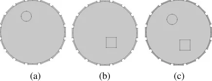
The samples used to learn the initial dictionary are constructed with COMSOL Multiphysics software. Three kinds of training data are created, as shown in Figure 1. The imaging area of the model is a circular area with a radius of 1 cm. A circular inclusion is simulated, with a radius on 0.16 and center values in the closed interval [0, 0.6]. A square inclusion is simulated, with side length of 0.32 and center values in the closed interval [0, 0.6]. A circular and a square combination inclusions are simulated, with radius of 0.16, side length of 0.32, and the center in the interval [0, 0.6]. The resolution for the image is 32×32 (the actual number of pixels is 812). The number of different kinds of samples is same, which can avoid sample imbalance. The whole training datasetH includes 3627 images, in which every kind of dataset has 1209 images. According to the size of the target object in the training images, the patch size is chosen as 5×5, and the number of dictionary atoms is set toK = 60, M = 25. Each image is composed of 576 patches, and as a consequence, over 2 million patches are obtained based on 3267 images for sample data which constitute X in Equation (6).
In this section, we mainly optimize the model by adjusting the learning rate and the number of iterations. As for dictionary learning, learning rate is an important factor to be considered. The learning
(a) (b) (c)
rate is set to 0.02, 0.2, and 0.1. The number of iterations of reconstruction also significantly affects image quality. Keep the number of iterations fixed when optimizing the learning rate, and keep the learning rate fixed when optimizing the number of iterations. 1% level of noise is added to the simulated voltages for testing the noise robustness of the new method.
EIT image is reconstructed based on the dictionary learning algorithm discussed in Section 2, and the conductivity distribution is obtained by measuring the changes in voltage. RLS-DLA is used to learn an initial dictionary with prior information, using Equations (10) and (11) to update the dictionary. Difference image, position error (PE), and shape deformation (ΔS) are adopted to effectively evaluate EIT image quality [23]. We define
P E= rt−r0
r0 (14)
wherer0 is the distance from the center of the target to the origin in the true-value image, andrt is the distance from the Center of Gravity (COG) of the target to the origin in the reconstructed image. ΔS
is a parameter used to evaluate the shape deformation of the target object in the reconstructed image, which can be expressed as
ΔS= Nt−N0
N0 (15)
whereNtis the number of pixels in a given threshold of the reconstructed image, andN0 is the number of pixels in the true-value image whose value is 1.
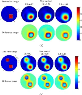
Two models are simulated to test the new method. PE, ΔS, and difference image are used to evaluate the image quality. In Figure 2, comparing the results at different learning rates (LR) when the number of iterations is fixed to 4 times, PE and ΔS of two methods are shown in Table 1. In this
(a)
(b)
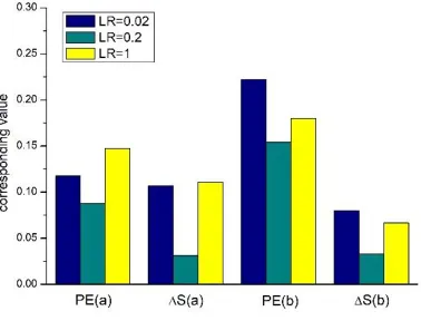
Table 1. PE and ΔS of the new method at different learning rates. New method
LR = 0.02 LR = 0.2 LR = 1 PE (a) 0.1176 0.0877 0.1476 ΔS (a) 0.1067 0.0311 0.1111 PE (b) 0.2223 0.1542 0.1799 ΔS (b) 0.0800 0.0333 0.0667
Table 2. PE and ΔS of the new method at different number of iterations. New method
n= 2 n= 6 n= 10 n= 14
PE (a) 0.1476 0.1298 0.1148 0.1778 ΔS (a) 0.1111 0.0400 0.0044 0.3333 PE (b) 0.1664 0.1213 0.0923 0.0991 ΔS (b) 0.0733 0.0433 0.0200 0.0867
experiment, the threshold used to calculate ΔS is set to 0.62, which means that we calculate ΔS in a region where the pixel value is greater than 0.62.
From Figure 2, the difference images illustrate that both LR = 0.02 and LR = 1 still cause a number of artifacts in homogeneous regions where the signal magnitude is zero. And both of them correspond to larger errors in the region where the signal magnitude is equal to one. We can see from Table 1 and Figure 3 that both the PE and ΔS obtain the smallest value when LR = 0.2. So we fix the initial dictionary with LR = 0.2 to discuss the number of iterations (expressed as n), and the result is shown in Figure 4 and Table 2.
Figure 3. The bar graph associated with Table 1.
In Figure 4, whenn= 10, we get the best visual effect with the fewest artifacts, and the difference image corresponds to the smallest error in all regions. It can be seen from Table 2 and Figure 5 that as the number of iterations increases to 10, PE and ΔS become smaller and smaller, but continuing to increase the number of iterations will result in larger PE and ΔS. Therefore, in the following simulation experiment, for the new method, we fix the initial dictionary D0 with LR = 0.2 and fix the number of iterations n= 10.
(a)
(b)
Figure 4. Reconstructed images obtained from simulated voltage data with different number of iterations. (a) The model of one square and (b) the model of a circle and a square are simulated.
Figure 5. The bar graph associated with Table 2.
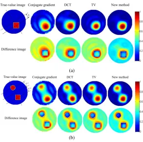
method [24] are compared with that of patch-based sparsity method based on fixed DCT initial dictionary and RLA-DLA initial dictionary. As can be observed from Figure 6, new method shows better performance in both artifacts suppression and details preservation. We can see that the conjugate gradient method is seriously affected by the ill-posedness so that the error is large. DCT and TV perform better than CG but still worse than the new method. The difference image of the new method obviously corresponds to the smallest value in all regions. We know that PE and ΔSare important characteristics for EIT. From Table 3 and Figure 7, the new method obtains minimum value of two parameters, which means that the new method is superior to the other two in terms of positioning and shape recovery of the target object.
(a)
(b)
Figure 6. Reconstructed images of (a) the model of one square and (b) the model of a circle and a square are obtained from simulated voltage data with four different methods.
Table 3. Comparison of the four methods in terms of PE and ΔS.
CG DCT TV New method PE (a) 0.3400 0.1600 0.1480 0.1148 ΔS (a) 0.3644 0.2133 0.1856 0.0044 PE (b) 0.2832 0.1544 0.1333 0.0923 ΔS (b) 0.1133 0.0533 0.0500 0.0200
while the convergence rate of new method is greatly increased because of using the initial dictionary with prior information.
5. EXPERIMENTAL RESULTS WITH REAL DATA
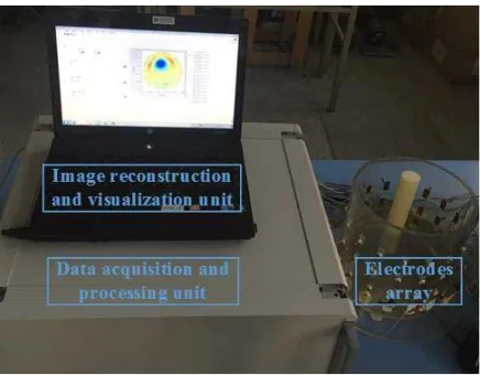
An EIT system has been developed by our group, as shown in Figure 9. In the data acquisition and control system, AC-based sensing electronics is composed of the resistor voltage (R/V) converter and AC programmable gain amplifier (AC-PGA). The digital signals are captured and processed by the FPGA (Xilinx Spartan3XC3S400), including digital phase-sensitive demodulation (digital PSD), and first-in, first-out (FIFO). The data acquisition speed of the system is approximately 30 frames/s. Sixteen composite electrodes are evenly distributed on the inner surface of the container. Adjacent currents injected from a single current source and adjacent voltage measurement strategies are used. 0.3 mA sinusoidal current signal is used for excitation, and all measurements are made at 3 kHz. The voltage values on the adjacent electrodes are measured and circulated in sequence until all of them are excited, resulting in 208 measured voltage values.
Figure 7. The bar graph associated with Table 3.
(a) (b)
Figure 8. Comparison of convergent rate between DCT fixed dictionary method and new method, (a) the model of one square; (b) the model of a circle and a square.
water (0.42 Sm−1) to a height of 10 cm to serve as the material of the image background. Four agar robs are used in the experiment, and the cross-section shapes are circular (diameterd= 3 cm,d= 6 cm) and square (side length a= 3 cm,a= 6 cm). The conductivities of all agar rods are 0.71 Sm−1.
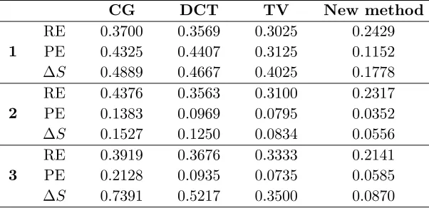
As shown in Figure 10, three groups of real data experiments have been implemented. In the experiments, the new method is compared with the CG, DCT dictionary methods and TV method in terms of RE (relative error), PE, and ΔS. The optimal initial dictionaryD0 obtained in the simulation experiment is applied in the new method, and the number of iterations n = 10 is chosen for image reconstruction.
From Figure 10 we can see that the new method can remove artifacts superior to the conjugate gradient method, DCT dictionary metho,d and TV method, and Table 4 shows that the new method not only can get the smallest RE but also performs best in positioning and recovering the target shape.
Figure 10. Image reconstruction of experiments.
Table 4. Comparison of the four methods in terms of RE, PE and ΔS.
CG DCT TV New method
1 RE PE ΔS 0.3700 0.4325 0.4889 0.3569 0.4407 0.4667 0.3025 0.3125 0.4025 0.2429 0.1152 0.1778 2 RE PE ΔS 0.4376 0.1383 0.1527 0.3563 0.0969 0.1250 0.3100 0.0795 0.0834 0.2317 0.0352 0.0556 3 RE PE ΔS 0.3919 0.2128 0.7391 0.3676 0.0935 0.5217 0.3333 0.0735 0.3500 0.2141 0.0585 0.0870 6. CONCLUSIONS
60%, 41%, and 30% compared to CG, DCT, and TV methods. The relative error is reduced by more than 30% compared to traditional methods. As for the convergence rate, the new method improves 37% compared to DCT method. Both simulated and experimental results illustrate the effectiveness of the new method.
ACKNOWLEDGMENT
This research is funded by the National Natural Science Foundation of China (61872269, 61601324 and 61903273), Natural Science Foundation of Tianjin Municipal Science and Technology Commis-sion (18JCYBJC85300), Tianjin Enterprise Science and Technology Correspondent Project (18JCT-PJC61600 and 18JCTPJC59000) and Tianjin Science and Technology Program (19PTZWHZ00020).
REFERENCES
1. Wang, Q., et al., “Reconstruction of EIT images via patch based sparse representation over learned dictionaries,” Instrumentation & Measurement Technology Conference, IEEE, 2015.
2. Goharian, M., M. Soleimani, and G. R. Moran, “A trust region subproblem for 3D electrical impedance tomography inverse problem using experimental data,” Progress In Electromagnetics Research, Vol. 94, 19–32, 2009.
3. Vauhkonen, M., et al., “Tikhonov regularization and prior information in electrical impedance tomography,”IEEE Transactions on Medical Imaging, Vol. 17, No. 2, 285–293, 1998.
4. Oraintara, S., “A method for choosing the regularization parameter in generalized tikhonov regularized linear inverse problems,”Int. Conf. Image Process, Vol. 1, 2000.
5. Tian, W., M. F. Ramli, W. Yang, and J. Sun, “Investigation of relaxation factor in landweber iterative algorithm for electrical capacitance tomography,” 2017 IEEE International Conference on Imaging Systems and Techniques (IST), 1–6, Beijing, 2017.
6. Baloch, G. and H. Ozkaramanli, “Image denoising via correlation-based sparse representation,”
Signal, Image and Video Processing, 2017.
7. Quan, X., et al., “Image denoising based on adaptive over-complete sparse representation,”Chinese Journal of Scientific Instrument, Vol. 30, No. 9, 1886–1890, 2009.
8. Elad, M. and M. Aharon, “Image denoising via sparse and redundant representations over learned dictionaries,” IEEE Transactions on Image Processing, Vol. 15, 3736–3745, 2006 (Pubitemid 44811686).
9. Rubinstein, R., et al., “Dictionaries for sparse representation modeling,” Proceedings of the IEEE, Vol. 98, No. 6, 1045–1057, 2010.
10. Wang, J., et al., “Split Bregman iterative algorithm for sparse reconstruction of electrical impedance tomography,”Signal Processing, Vol. 92, No. 12, 2952–2961, 2012.
11. Aharon, M., M. Elad, and A. Bruckstein, “K-SVD: An algorithm for designing overcomplete dictionaries for sparse representation,” IEEE Transactions on Signal Processing, Vol. 54, No. 11, 4311–4322, 2006.
12. Engan, K., K. Skretting, and J. H. Husøy, “A family of iterative LS-based dictionary learning algorithms, ILS-DLA, for sparse signal representation,” Digital Signal Processing, Vol. 17, 32–49, Jan. 2007.
13. Mailh´e, B., S. Lesage, R. Gribonval, and F. Bimbot, “Shift-invariant dictionary learning for sparse representations: Extending K-SVD,” Proceedings of the 16th European Signal Processing Conference (EUSIPCO2008), Lausanne, Switzerland, Aug. 2008.
14. Mairal, J., F. Bach, J. Ponce, and G. Sapiro, “Online dictionary learning for sparse coding,”
ICML’09: Proceedings of the 26th Annual International Conference on Machine Learning, 689– 696, ACM, New York, NY, USA, Jun. 2009.
16. Jin, B., T. Khan, and P. Maass, “A reconstruction algorithm for electrical impedance tomography based on sparsity regularization,” International Journal for Numerical Methods in Engineering, Vol. 89, No. 3, 337–353, 2012.
17. Gong, B., et al., “Sparse regularization for EIT reconstruction incorporating structural in formation derived from medical imaging,” Physiological Measurement, Vol. 37, No. 6, 843–862, 2016.
18. Wang, Q., et al., “Patch based sparse reconstruction for electrical impedance tomography,” Sensor Review, Vol. 37, No. 3, 2017.
19. Fan, W., et al., “Modified sparse regularization for electrical impedance tomography,” Review of Scientific Instruments, Vol. 87, 2016.
20. Zhao, B., H. X. Wang, X. Y. Chen, X. L. Shi, and W. Q. Yang, “Linearized solution to electrical impedance tomography based on the Schur conjugate gradient method,”Measurement Science and Technology, Vol. 18, No. 11, 3373–3383, 2007.
21. Skretting, K. and K. Engan, “Image compression using learned dictionaries by RLS-DLA and compared with K-SVD,” IEEE International Conference on Acoustics, IEEE, 2011.
22. Press, H., S. A. Teukolsky, W. T. Vetterling, and B. P. Flannery, “Section 2.7.3. Noodbury Formula,”Numerical Recipes: The Art of Scientific Computing, 3rd Edition, Camdridge University Press, New York, ISBN 978-0-521-88068-8, 2007.
23. Adler, A., et al., “GREIT: A unified approach to 2D linear EIT reconstruction of lung images,”
Physiological Measurement, Vol. 30, No. 6, S35–S55, 2009.