AVR, AZHAGAN. Characterizing Driving Behavior by using LIDAR and GPS through Traffic Stream Models. (Under the direction of Drs. Rachana Gupta and Nagui Rouphail).
© Copyright 2019 by Azhagan Avr
by Azhagan Avr
A thesis submitted to the Graduate Faculty of North Carolina State University
in partial fulfillment of the requirements for the degree of
Master of Science
Electrical Engineering
Raleigh, North Carolina 2019
APPROVED BY:
_______________________________ _______________________________ Dr. Rachana Gupta Dr. Nagui Rouphail
Co-Chair of Advisory Committee Co-Chair of Advisory Committee
_______________________________ _______________________________ Dr. Donna Yu Dr. Shams Tanvir
ii
DEDICATION
I dedicate this work to my parents Manjari Avr and Raviraj Jambulingam, and my sister Anjana Avr and my friends from LICET and NCSU for their never-ending support and belief in me.
iii BIOGRAPHY
Azhagan Avr was born and brought up in Chennai, India. He did his schooling in St. Michael’s Academy, Chennai, India. In the year 2016 he graduated with an undergraduate degree in Electronics and Communication from Loyola ICAM – College of Engineering and Technology (LICET) affiliated to Anna University, Chennai, India. His interests in projects and excellence in academics earned him an opportunity to be an exchange student at Comillas Pontifical University, Madrid, Spain in June 2015. As a research scholar, he performed a month-long research in amplifier stability. In February 2016, he was given an opportunity to perform his final year project in Hochschule Heilbronn, Heilbronn, Germany. He worked on integrating an industrial Laser scanner in an autonomous farming vehicle.
iv
ACKNOWLEDGMENTS
This thesis presents my contribution in Characterizing Driving Behavior by using LIDAR and GPS through Traffic Stream Models. This research was an extension of the ARPA-E project carried out at ITRE.
I would like to thank Dr. Nagui Rouphail and Thomas Chase for trusting me and giving me the opportunity to work on the ARPA-E project. Dr. Rouphail has been a constant guidance throughout my research and I would like to express my gratitude for his patience, enthusiasm and for sharing his immense knowledge. Dr. Shams Tanvir has played a vital role in my entire thesis and has always been available to answer any questions that I have had and has always made time for me and been patient in explaining the technical nuances.
My sincere thanks to my advisor Dr. Rachana Gupta who has guided me towards achieving the end goal of completing my thesis. She has been very kind, and our conversations and discussions have always made me feel at home. I would also like to thank Dr. Ginger Yu who has guided me in choosing the most suitable coursework to accompany my thesis.
v
TABLE OF CONTENTS
LIST OF TABLES ... viii
LIST OF FIGURES ... ix
1 INTRODUCTION ... 1
1.1 Problem Definition and Motivation ... 1
1.2 Literature Review ... 3
1.3 Methodology ... 5
1.4 Structure of the Thesis... 6
2 SYSTEM INTEGRATION AND DATA COLLECTION ... 7
2.1 Introduction ... 7
2.2 System Components ... 7
2.2.1 Light Detection and Ranging (LIDAR) ... 7
2.2.2 Global Positioning System (GPS) ... 8
2.2.3 Real Time Clock (RTC) ... 8
2.2.4 Camera ... 9
2.2.5 Laser Pointer ... 10
2.2.6 Arduino ... 10
2.2.7 Raspberry Pi ... 11
2.2.8 Mount ... 12
2.2.9 System Architecture ... 12
2.3 Data Collection ... 13
2.3.1 Route Details ... 14
2.3.2 Data ... 16
3 DATA FILTERING AND ERROR ANALYSIS ... 17
3.1 Introduction ... 17
3.2 Simple Exponential Smoothing (SES) ... 17
3.3 Auto Regressive Integrated Moving Average (ARIMA) ... 17
3.4 Mean Filter ... 19
3.5 Data Filtering Algorithm ... 20
3.6 Error Analysis ... 21
vi
4 TRAFFIC STREAM MODELS ... 26
4.1 Introduction ... 26
4.2 Microscopic Traffic Models ... 26
4.2.1 Wiedemann Car-Following Model ... 26
4.3 Macroscopic Models ... 29
4.3.1 Local Density ... 29
4.3.2 Speed vs Density ... 30
4.3.3 Standard macroscopic models... 30
5 DATA ANALYSIS AND RESULTS ... 32
5.1 Introduction ... 32
5.2 Trip Characteristics ... 32
5.2.1 Arterial Trip Data ... 32
5.2.2 Freeway Trip Data ... 34
5.2.3 Trip Statistics ... 34
5.3 Longitudinal Evolution of Density ... 36
5.3.1 Arterial Route... 36
5.3.2 Freeway Route ... 37
5.3.3 Trip Statistics ... 37
5.4 Speed vs Density vs Wiedemann Model ... 39
5.4.1 Arterial Route... 39
5.4.2 Freeway Route ... 40
5.4.3 Trip Statistics ... 41
5.4.4 Application and Correlation ... 42
5.5 Speed vs Density vs Standard Models ... 43
5.5.1 Arterial Route... 43
5.5.2 Freeway Route ... 46
5.5.3 Application and Correlation ... 48
6 CONCLUSION AND FUTURE WORK ... 49
6.1 Goals and Objectives ... 49
6.2 Major Findings ... 50
6.3 Impact ... 50
6.4 Limitations ... 51
vii
viii
LIST OF TABLES
Table 2.1: Sample Dataset ... 16
Table 3.1: Mean Square Error Analysis ... 22
Table 5.1: Trip Statistics ... 35
Table 5.2: Longitudinal Variation of Local Density across Sub-Segments... 38
Table 5.3: Trip Statistics ... 41
Table 5.4: Fitted Traffic Model Parameters - Arterial ... 45
ix
LIST OF FIGURES
Figure 2.1: LIDAR-Lite v3 ... 7
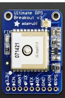
Figure 2.2: Adafruit Ultimate GPS ... 8
Figure 2.3: DS3231 Real-Time Clock ... 8
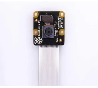
Figure 2.4: Raspberry Pi Camera ... 9
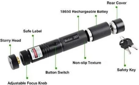
Figure 2.5: Laser Pointer... 10
Figure 2.6: Arduino Uno Microcontroller ... 10
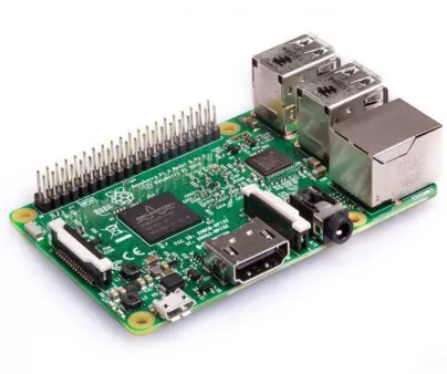
Figure 2.7: Raspberry Pi 3 Model B ... 11
Figure 2.8: Delkin Fat Gecko Suction Mount ... 12
Figure 2.9: System Architecture ... 12
Figure 2.10: (a). LIDAR affixed on the hood of the car (b). Snapshot from the video. ... 14
Figure 2.11: Arterial Route ... 14
Figure 2.12: Freeway Route ... 15
Figure 3.1: Illustrates the change in car-following events. ... 18
Figure 3.2: Illustrates the raw data from the LIDAR for the scenarios shown in Figure 3.1. ... 19
Figure 3.3: Shows a Flowchart of the 2 step-filtering process ... 21
Figure 3.4: Compares ground truth values with predicted and filtered data. ... 23
Figure 3.5: Route traveled for collecting the data... 23
Figure 3.6: (a). Snapshots (b). highlights the noisy sections (c). ARIMA (0,1,1) prediction ... 24
Figure 3.7: The plot shows the fully processed output ... 25
Figure 4.1: Regime thresholds of the Wiedemann model [16]. ... 27
Figure 4.2: Greenshields Model ... 30
Figure 4.3: Modified Greenberg Model ... 31
Figure 5.1: Sample data collected during PM peak on the arterial segment. ... 33
Figure 5.2: Sample data collected during PM peak on the Freeway segment. ... 34
Figure 5.3: Local density profile across the arterial segment in the PM peak. ... 36
Figure 5.4: Local density profile across the freeway segment in the PM peak. ... 37
Figure 5.5: Instantaneous Speed-Local Density with Wiedemann Regimes for Arterial ... 39
x
1
1
INTRODUCTION
1.1 Problem Definition and Motivation
In the 1970s, ropes were used to measure the spatial gap between vehicles. But, nowadays with advances in technologies, these are collected through a variety of state-of-the-art techniques. Researchers have used video data to identify the gap between vehicles [1]. Some researchers have used GPS data for speed capturing but also for estimating the gap between vehicles using positional data [2]. But in the techniques mentioned above, the spatial gap between vehicles is being estimated and not captured; hence there is always scope for inaccuracy in such techniques.
Hence a probable solution to collect the gap between vehicles would be using sensors like Light Detection and Ranging (LIDAR) or Radio Detection and Ranging (RADAR). At present, almost all new vehicles are equipped with sensors like LIDAR or RADAR for Advanced Driver Assistance Systems (ADAS). But data from these sensors are not accessible to users through the On-Board Diagnostics (OBD) port. Hence this research would be useful for future studies that use vehicles to collect spatial gap between vehicles like car-following data for various research practices.
One of the common methods of collecting traffic flow and vehicle volume data in a segment is through static or stationary infrastructure sensors. Some of the commonly used methods of data collection are stationary video cameras or vehicle counting sensors like the Remote Traffic Microwave Sensor (RTMS) [3]. These methods, however, lack variation in space over the segment as the sensors are fixed to a location and the collected data is usually averaged out to estimate the information about the entire segment. That is often the reason macroscopic models use average speed and average density. Also, Installations and reinstallations of these stationary sensors in different locations are expensive and difficult to maintain [4].
An alternative solution to collect data in a cost-effective way would be through a dynamic method where the sensor is in motion. Some researchers have used devices that collect vehicular speed data from the On-Board Diagnostics (OBD) port [5], and some have used Global Positioning System (GPS) devices to log vehicular speed and positional data from probe vehicles [6]. But these dynamic methods of data collection cannot report vehicle volume or occupancy information.
2
between vehicles from a moving vehicle. This can be achieved by using LIDAR or RADAR. Similar setups are found on commercially available autonomous vehicles (AV). Nowadays vehicles are equipped with different sensors to provide different information to the driver, like LIDARs are used to detect and measure the distance of objects or vehicles from an AV [7] and GPS modules are used in the in-built navigations systems for positional data. LIDAR and RADAR can be expensive, but this study uses a low-cost way to collect spatial gap between vehicles using LIDAR. From the instantaneous spatial gap between vehicles captured, “local density” can be calculated, along with the characterization of the entire lead vehicle trajectory while that vehicle is in range.
The local density is generated based on the driver’s reactions to the leading vehicle, that is, the dynamic data collected pertaining to the driver of the following (equipped) vehicle across the corridor. The advantage of the naturalistic approach is that information is collected without any bias or any controlled conditions. One purpose of this research is to demonstrate the effectiveness of this approach.
The motivation for this research is to develop a low-cost, dynamic and a prototype with good accuracy that would capture spatial gap between vehicles, unlike the traditional stationary devices that capture gap between vehicles information from stationary positions. The main motivation of this research was to capture data in an independent, naturalistic and dynamic way and characterize the driving behavior with the captured gap between vehicles and vehicular speed. Some of the questions that motivated me to pursue my research on this topic are listed below;
a) Can a low-cost LIDAR capture accurate reading while in motion? b) Is the chosen ARIMA model the most appropriate to the application? c) Are the results of the 2-stage filtering process promising?
d) What is the need for local density data through dynamic data collection?
e) How does classifying speed-density data into regimes help in characterizing driving behavior? f) Can some of the existing macroscopic models represent the dynamic data?
3
1.2 Literature Review
As mentioned in the previous section, various techniques have been used to estimate the spatial gap between vehicles. An image processing tool used to classify vehicles in a mixed traffic scenario is used to estimate the spatial gap between vehicles [1]. But the disadvantage of using cameras for measuring the gap between vehicles is that the camera needs to be calibrated for every location the camera is being installed, the following study shows a method that can be used to calibrate the camera [8], which is an added challenge. Apart from calibration, there are other challenges faced when stationary sensors are used like restrictions on installations, environmental factors and cost of installations and reinstallations [4]. Hence dynamic data-driven methods are the way to move forward [9].
An alternative solution to stationary sensors could be using GPS devices to estimate the spatial gap between vehicles. The research proposes that positional and speed data obtained from GPS traces are cost-effective and accurate [10]. Using the positional data of two known vehicles the gap between vehicles is estimated [2]. This method of dynamic data collection brings in the factor of dependency on the data from the leading vehicle which rules out collecting data from different commercial users independently, as at any given time 2 vehicles are needed for data collection.
In the methods mentioned above the spatial gap between vehicles, are not captured directly but they are estimated. Hence the methodology used in this research involves a naturalistic approach of data collection that is independent of other vehicles for the data.
RADAR and LIDAR both have a similar functionality except that LIDAR uses light waves and RADAR uses radio waves to measure distance. Both these devices have their set of advantages and disadvantages, but both the sensors are widely used in the latest vehicles [11] for ADAS. This research uses a LIDAR device for measuring the distance.
4
the 2D sensor with the intended application, the 1D sensors were later considered. 1D sensors do not map the environment, nor rotate 360 degrees, but they produce a singular light beam at a frequency between 500 – 1000 Hz which is then bounced of the surface of the leading vehicle and the reflected beams are captured and distance is measured. They are less expensive compared to the other LIDAR devices, the LIDAR used here is priced at $125 and the device is small, low power and compact.
ARIMA is a prediction model that is used for time series forecasting [12]. The model can predict a value based on the selected range of values. ARIMA is used to predict the spatial distance between cars. The mean filter also known as an averaging filter is used to filter the data that is rejected by the ARIMA prediction.
Various methods have been employed to collect microscopic information like speed and headways and macroscopic information like vehicle occupancy, vehicle flows, and so on with static sensors. One such method was to use an offline image processing tool to classify vehicles in a mixed traffic scenario and gather microscopic information like speed and headway and macroscopic characteristics like vehicle trajectories, vehicle occupancy, and so on [3]. The drawbacks of similar systems are that the area covered by theses sensors is only hundreds of feet wide i.e. they lack spatial variation over the segment and the installation and maintenance cost would be expensive as well.
5
The car is assumed to be following when the driver is unable to drive at the desired speed and is constrained by the leading vehicle [16]. The car-following model being used is a psycho-physical model designed by VISIM also called a Wiedemann model. The enhanced version of the 1974 model, proposed by Wiedemann and Reiter in 1992 [17]. Wiedemann model being a microscopic car-following model that is entitled to a single driver’s behavior makes use of dynamic information such as headway, speed of the follower and speed of the leader vehicle. In Wiedemann car-following model, the thresholds are defined for every speed, so it helps to identify the driving behavior at different speeds [18]. Through this model, each data point is categorized into a regime.
Various macroscopic models like Greenshields, Modified Greenberg, etc. are used for investigating the quality and closeness of the dynamic speed-density data. These models are usually fitted to data that are collected using static sensors over time at a given location with temporal variation but lacking variation in space over the segment. This research explores how the models would represent dynamic data.
Hence from the literature mentioned above, some systems that capture speed and vehicle occupancy from static locations lack the evolution of density in space. Some dynamic systems with GPS or OBD devices capture speed data but do not capture density data. But methods used to collect speed and density data from the GPS requires a controlled environment and are dependent on other vehicles to house similar data capturing devices to obtain speed and density data. Hence this research proposes to use LIDAR and GPS to capture the gap between vehicle and speed of the equipped vehicle, respectively.
1.3 Methodology
This research discusses a cost-effective method to collect the distance between two vehicles using LIDAR, and a method to process and filter the outliers from the raw data. A 2-stage process which involves ARIMA prediction modeling in stage 1 and mean-filtering in stage 2 to filter out the noise in the raw data from the sensor. When the manufacturers make the raw sensor data available to users through the OBD port, the same method of noise removal can be implemented, but due to its unavailability, an external sensor is used.
6
domain into different car-following regimes and (c) a comparison of various traditional macroscopic models with the collected speed-local density data. In fact the data streams generated in this work resemble those likely to be produced by autonomous and connected vehicles, thus providing a preview of possible applications of such data for enhanced mobility and safety purposes.
1.4 Structure of the Thesis
7
2
SYSTEM INTEGRATION AND DATA COLLECTION
2.1 Introduction
In this chapter, the components that were used to develop the device are discussed in detail with their usage and specifications. Then the data collection process and routes are explained. Finally, the different data sets obtained through this process are briefed.
2.2 System Components
In this section, the component specifications and the device architecture are explained.
2.2.1 Light Detection and Ranging (LIDAR)
Figure 2.1: LIDAR-Lite v3
8 2.2.2 Global Positioning System (GPS)
Figure 2.2: Adafruit Ultimate GPS
The breakout board is built around the MTK3339 chipset, with a high-quality GPS module that can track up to 22 satellites on 66 channels, has an excellent high-sensitivity receiver (-165 dB tracking), and a built-in antenna. It can do up to 10 location updates a second (10Hz) for high speed, high sensitivity logging, or tracking. Power usage is incredibly low, only 20 mA during navigation. The Breadboard Breakout board comes with an ultra-low dropout 3.3V regulator. A footprint for optional CR1220 coin cell to keep the RTC running and allow warm starts and a tiny bright red LED. The LED blinks at about 1Hz while it's searching for satellites and blinks once every 15 seconds when a fix is found to conserve power .
2.2.3 Real Time Clock (RTC)
Figure 2.3: DS3231 Real-Time Clock
9
input and maintains accurate timekeeping when the main power to the device is interrupted, in this case, it maintains the time when the Raspberry pi is switched off. The integration of the crystal resonator enhances the long-term accuracy of the device as well as reduces the piece-part count in a manufacturing line. The RTC maintains seconds, minutes, hours, day, date, month, and year information. The date at the end of the month is automatically adjusted for months with fewer than 31 days, including corrections for leap year. The clock operates in either the 24-hour or 12-hour format with an AM/PM indicator .
2.2.4 Camera
Figure 2.4: Raspberry Pi Camera
10 2.2.5 Laser Pointer
Figure 2.5: Laser Pointer
A laser pointer was used during the research while installing the external LIDAR sensor on the hood of the vehicle.
2.2.6 Arduino
Figure 2.6: Arduino Uno Microcontroller
11
support the microcontroller; simply connect it to a computer with a USB cable or power it with an AC-to-DC adapter or battery to get started. The Uno board is the first in a series of USB Arduino boards and the reference model for the Arduino platform .
2.2.7 Raspberry Pi
Figure 2.7: Raspberry Pi 3 Model B
12 2.2.8 Mount
Figure 2.8: Delkin Fat Gecko Suction Mount
A Delkin Fat Gecko mount with dual suction cups was used to temporarily fix the LIDAR on to the hood of the vehicle during data collection.
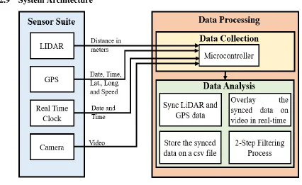
2.2.9 System Architecture
Figure 2.9: System Architecture
13
timestamps, speed, and positional data. The real-time clock is for updating the system time in the Raspberry pi and the video data from the camera is used as a reference to verify the data. The data output from the different devices is sent to the Data Processing unit which is a combination of an Arduino and Raspberry Pi. The Arduino receives the data captured from the GPS and LIDAR modules, organizes and syncs them together. The LIDAR has a range of 40 m and the output from the LIDAR module is in the form of pulses, whose width is converted to distance. The pulse width is expressed in the unit µs, 10 µs = 1 cm. The distance of the object in meters is,
Distance, d = Pulse width
1000 meters (1)
The Raspberry Pi performs the overlay of the GPS and LIDAR data on the video and stores the captured data in the CSV file. The 2-step filtering process can also be performed on the Raspberry Pi, but for convenience, visualization and efficiency of processing a large amount of data a separate laptop was used. The total cost of the entire setup would round up to $300.
2.3 Data Collection
During data collection, the LIDAR is mounted on the hood of the car using a specially made mount, which helps in the installation process. The mount consists of 2 suction pads, a shaft, and an aluminum panel with a laser pen holder.
14
Figure 2.10: (a). LIDAR affixed on the hood of the car (b). Snapshot from the video.
As seen in Figure 2.10a, the LIDAR is connected to the in-vehicle unit through wiring, which consists of components like Arduino, Raspberry Pi, Real-time clock, GPS and Camera. The in-vehicle unit is powered through the 12V cigarette lighter port. Data is collected by following random vehicles in different traffic conditions like congested and free flow driving situations on freeways and arterial roads.
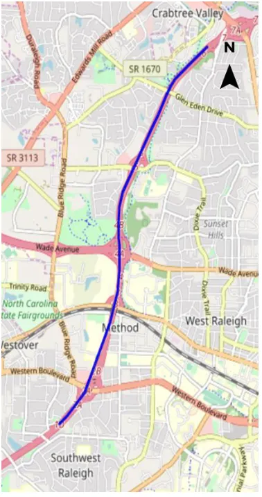
2.3.1 Route Details
The data was collected by naturalistic driving in two routes. The chosen routes consist of one arterial segment and one freeway segment.
Figure 2.11: Arterial Route
15
There are totally 8 signalized intersections with 2 on Gorman and 6 on Hillsborough street. Hillsborough Street has 4 roundabouts across the segment.
Figure 2.12: Freeway Route
16 2.3.2 Data
Through the developed low-cost system two forms of data were captured and stored, which are explained in the following sections.
2.3.2.1 Video Data with Overlay
The other data form stored in the Raspberry Pi is the video overlaid with the date (GPS), time (GPS), the spatial gap between vehicles (LIDAR), follower speed (GPS), and trip id. These variables are displayed on the video for reference which is highlighted in Figure 2.10b.
2.3.2.2 GPS – LIDAR Data
The GPS and LIDAR data captured from the respective modules are synced within the Arduino and then sent to the Raspberry Pi where data is stored in a CSV file. A sample of the data is shown below.
Table 2.1: Sample Dataset
Date Time Latitude Longitude Speed
(MPH)
Distance (meter)
Trip Id 2/19/2019 08:53:08 AM 35.770103 -78.682135 4 3.91 2 2/19/2019 08:53:08 AM 35.770103 -78.682135 4 3.95 2 2/19/2019 08:53:08 AM 35.770103 -78.682135 4 3.99 2 2/19/2019 08:53:08 AM 35.770103 -78.682135 4 0.14 2 2/19/2019 08:53:09 AM 35.770103 -78.682135 4 3.92 2 2/19/2019 08:53:09 AM 35.770103 -78.682135 4 3.98 2
The first and second column of Table 2.1 consists of the date and time, the third and fourth column consists of the vehicle’s latitude and longitude, 5th column is the speed of the vehicle in
17
3
DATA FILTERING AND ERROR ANALYSIS
3.1 Introduction
This chapter discusses the types of noises in the data and methods to remove the noises. Also, error analysis is performed to highlight the performance of the prediction modeling used for filtering and the accuracy of the LIDAR sensor. Finally, stagewise results of the filtering process are explained.
3.2 Simple Exponential Smoothing (SES)
The exponential smoothing window is used to smoothen the time series data. The past values are given equal weight in a moving average window, but in simple exponential smoothing, weights are exponentially increased over time [19]. The exponentially increasing weights help in providing less weight to the values away from the data point of interest [20]. Exponential smoothing is given by equation [19]:
St= α ⋅ xt+ (1 − α) ⋅ st−1= st−1+ α ⋅ (xt− st−1) (2)
where α is the smoothing factor with values from 0 < α < 1. St is the weighted average of the most recent observation xt and st−1 is the previously smoothed data. Large values of α provide greater weight to recent changes in the data, while small values of α are less responsive to recent changes. Hence the value of α depends on the data and the application. In this research, the simple exponential smoothing model is responsive to recent changes because each measured reading is independent of the previous readings i.e. the past values do not have an impact on present reading.
3.3 Auto Regressive Integrated Moving Average (ARIMA)
18
is considered as a noisy reading and sent to the next stage for filtering. Noises are of three types, namely, system noise that is caused by weak signals received after reflection from the vehicle, noise due to objects in the environment like trees, bushes, lamp posts, and noise due to change in car-following events, etc.
Figure 3.1: Illustrates the change in car-following events.
19
3.4 Mean Filter
As mentioned earlier, a sudden change in the spatial gap between vehicles can be due to weak signals or random objects or due to change in the car-following events. These types of readings are filtered out by ARIMA prediction modeling. Hence through mean filtering, the three types of readings are differentiated, and the change in car-following event readings (good noise) are retained, and the noise from random objects and system noise (bad noise) are discarded. The method of differentiating the readings is explained below;
Figure 3.2: Illustrates the raw data from the LIDAR for the scenarios shown in Figure 3.1.
With reference to Figure 3.1, Figure 3.2 illustrates the raw readings from the LIDAR module. The readings at t6, t8, and t9 are due to random objects, and reading at t7 is due to a weak reflected signal from the objects. The remaining data points are the reading of the vehicles. Readings captured from instant t0 to t5 are retained as valid data points by ARIMA prediction modeling. At t6 there is a sudden spike in data which is rejected by the ARIMA model, once rejected by the ARIMA model, mean filtering is performed, by averaging the values from t6 to t10. So, if the actual value at t6 is 17m but the average of the values from t6 to t10 is around 11.8 m, the difference between the actual value at t6 and averaged value is 5.2 m, so only when the difference between the actual value and the averaged value is less than 1m (threshold 2 as TH2) the value is retained. So, in this case, the value at t6 is discarded as a noisy value. Similarly, corresponding values from t7 to t9 are also discarded.
20
t10 to t14 is 20 m, and the difference between t10 and the average is less than 1m, so the sudden change in value is accepted as a valid data point. Similar processing happens in the transition from t19 to t20.
Hence through a combination of ARIMA prediction and mean filtering valid data points are retained, and invalid data points are discarded. The algorithm for this process is explained in detail below.
3.5 Data Filtering Algorithm
21
Figure 3.3: Shows a Flowchart of the 2 step-filtering process
3.6 Error Analysis
The main reason for choosing ARIMA (0,1,1) was its exponential smoothing model. Table 3.1 shows the error analysis between the different ARIMA models [22] commonly used for time series forecasting. To perform the error analysis, ground truth data were collected by physical measurements in a controlled environment.
22
MSE = 1
n∑ (yi− ŷ )i 2 n
i=1 (3)
Where n is the number of data points, yi is the observed value and ŷi is the predicted value.
The error analysis between ground truth and predicted value proves the accuracy of the ARIMA prediction with respect to the ground truth and the error analysis between the ground truth and the filtered data (final valid data points) proves the accuracy of the sensor with respect to the ground truth.
Table 3.1: Mean Square Error Analysis
ARIMA Model Ground Truth Vs
Prediction
Ground Truth Vs Filtered Data White Noise- (0,0,0) 17.28 meters 1.38 meters Random Walk- (0,1,0) 1.49 meters 0.98 meters
SES- (0,1,1) 0.13 meters 0.08 meters
1st order AR model- (1,0,0) 1.01 meters 0.96 meters
Differenced 1st order AR model-
(1,1,0) 1.08 meters 0.96 meters
LES- (0,2,1) 2.61 meters 1.39 meters
23
Figure 3.4: Compares ground truth values with predicted and filtered data.
In Figure 3.4, the blue dots denote the values captured by the LIDAR in real-time, the grey dots are the values predicted by ARIMA (0,1,1), and the orange dots are the actual ground truth values measured physically using measurement tools. Figure 3.4 verifies that the grey dots and the orange dots lie very close to each other, which proves the accuracy of the ARIMA (0,1,1) prediction model and similarly the orange and blue dots also lie close to each other, which proves the accuracy of the LIDAR.
3.7 Data Filtering Results
24
Figure 3.5 shows the trip map. The highlighted red route is the entire trip, the highlighted blue route is the section chosen for filtering. The three red dots are three instances of change in the car-following event. In the first instance the leading vehicle turns right eastbound on main campus drive, Raleigh, in the second event the leading vehicle turns left, northbound on Oval drive, Raleigh and in the third event the leading vehicle was turning left, westbound on Centennial Parkway, Raleigh.
The equipped vehicle was following the same leading vehicle before and after the change in car-following events. The route map is generated using the GPS data retrieved from the developed equipment. Following are the stage-wise results of the filtering process, the data shown below belongs to the blue line on the map.
Figure 3.6: (a). Snapshots (b). highlights the noisy sections (c). ARIMA (0,1,1) prediction
25
Figure 3.7: The plot shows the fully processed output
26
4
TRAFFIC STREAM MODELS
4.1 Introduction
In this research data is investigated and analyzed through microscopic and macroscopic models. This chapter explains the theory behind the microscopic and macroscopic models.
4.2 Microscopic Traffic Models
Microscopic traffic measures are commonly used to estimate macroscopic models and car-following models are a microscopic [16]. In this research, the Wiedemann car-car-following model and its usage are discussed in detail.
4.2.1 Wiedemann Car-Following Model
The two important information recorded in real-time are the gap between vehicles and speed of the following vehicle but, important information that is not measured in real-time would be the speed of the leading vehicle, which is estimated using the following formula;
Speed of the leader, vl = vf+ Δd
Δt, mile/hour (4)
Where vfis the instantaneous speed of the follower, Δd is the gap (rear bumper of the leading vehicle to the front bumper of the following vehicle) and Δt is the difference between time instances. The data collected can be visualized in various forms.
To implement the 1992 Wiedemann-Reiter car-following model, two important parameters are calculated [16]:
Headway, Δx = d + L, meters (5)
Where d is the gap (rear bumper of the leading vehicle to front bumper of the following vehicle) in meters and L is the length of the following vehicle in meters, and the difference in speed is;
27
Where vfis the instantaneous speed of the follower and vl is the speed of the leader in mile/hour. The VISIM or Wiedemann car-following model is the largest parameterized model when compared to the AIMSUN, MITSIM, and Fritzsche model [16]. So, using the above two parameters Δv, Δx along with certain calibration parameters, the thresholds for the VISIM car-following model are defined. There are in total 6 thresholds defined for this model.
Figure 4.1: Regime thresholds of the Wiedemann model [16].
AX would be the desired distance between two stationary vehicles;
AX = Ln−1+ AXadd + RND1n ∗ AXmult (7)
Where AXadd and AXmult are calibration parameters whose values are 1.25 and 2.5, respectively [16]. ABX is the desired distance between the leader and follower at low-speed differences;
28
BX = (BXadd + BXmult ∗ RND1n) ∗ √v (9)
v = {vl : νf > νl , vf : νl ≥ νf} (10)
Where BXadd and BXmult are calibration parameters, whose values are 2 and 1, respectively [16]. The maximum distance maintained by the follower in a car-following scenario is defined as SDX;
SDX = AX + EX ∗ BX (11)
EX = EXadd + EXmult ∗ (NRND − RND2n) (12)
Where EXadd and EXmult are calibration parameters, whose values are 1.5 and 0.55 [16]. SDV is the point where the driver realizes he/ she is approaching a slower vehicle;
SDV = (Δx−Ln−1−AX
CX )
2
(13)
CX = CXconst ∗ (CXadd + CXmult ∗ (RND1n + RND2n)) (14)
Where CXconst , CXadd and CXmult are calibration parameters; CX is rounded to 40 [16]. CLDV is the point where the driver realizes he/she is closing in on a slower vehicle and must decelerate to avoid a collision;
CLDV = SDV ∗ EX2 (15)
Finally, the OPDV threshold where the driver realizes that his/her speed is not constrained by the leading vehicle,
29
Where OPDVadd and OPDVmult are calibration parameters whose values are 1.5 and 1.5 respectively [16]. There are three normally distributed driver parameters namely
NRND, RND1n and RND2n, whose values are N(0.5,0.15) [16]. For all calculations, the mean value of 0.5 has been used.
As shown in Figure 4.1, when Δx vs Δv is plotted against the Wiedemann thresholds, each data point can be classified into a specific regime. There are totally 6 regimes namely; emergency, high density, following, approaching, closing-in and free driving regime. Emergency and high-density regime are low speed - low distance regimes. Data falls within emergency and high-high-density regimes regime when the speed of the follower is greater than the leader and lower than the speed of the leader respectively. Free driving and closing-in are high speed - high distance regimes, data that falls within these regimes are due to speed of follower is lower than the leader and higher than the leader respectively. Approaching regime is a transition phase between free driving and closing-in regimes. Fclosing-inally, followclosing-ing regime is centered between the other five regimes, data falls withclosing-in this regime when the leader and follower have very small speed differences. Hence each data point will belong to one of the six car-following regimes.
4.3 Macroscopic Models
Macroscopic traffic models are explained through the relationship between Flow, Density and Speed. This research focusses on the relationship between speed and density.
4.3.1 Local Density
The headway data (Δx) gives information about the car-following distance maintained by the follower at every instant, from which the average spatial distance over the segment can be measured. Like the speed of the leader vehicle, the local density is also estimated using the captured information with the formula as;
Local Density, DL=
1609.34
d+L Vehicles/mile (17)
30
distribution across the segment can be understood, unlike the stationary sensors which capture information only for a small portion of a segment.
The LIDAR device has a measurement limitation of 40m and considering the length of the following vehicle is 5m, local density less than 35 veh/mi cannot be measured. Based on the local density variation the driver's behavior pertaining to the environment and the traffic conditions can be studied.
4.3.2 Speed vs Density
With the Local density estimated, instantaneous speed – local density plots can be plotted to study their relation. At the y-intercept, density is zero and the speed is termed as Free-flow speed and at the x-intercept speed is zero and density is termed as jam density. Some standard speed-density models are explained in the following section.
4.3.3 Standard macroscopic models
Macroscopic traffic stream models like Greenshields and Modified Greenberg are used to investigate the quality of the dynamic data from the arterial and freeway segment based on their best-fit parameters. In Greenshields model, as shown in Figure 4.2 the speed-density relationship is expressed as [23];
u = uf(1 − k
kj) (18)
Where u, uf, k, and kj are the speed, free-flow speed, density, and jam density.
31
Unlike Greenshields, which is a single regime model, Modified Greenberg is a multi-regime model with 2 multi-regimes where the data is categorized into the free-flow and congested regime, as shown in Figure 4.3. For density values below kc the speed is free-flow speed uf, and the speed-density relation for density above kcis expressed as [23];
Figure 4.3: Modified Greenberg Model
u = um∗ ln (kj
32
5
DATA ANALYSIS AND RESULTS
5.1 Introduction
In this chapter, three methods of data investigations are discussed. Each method has a different perspective on driver behavior.
5.2 Trip Characteristics
As mentioned earlier various information such as headway, speed of follower, speed of the leader is obtained and Wiedemann car-following models are visualized to understand the actual traffic condition at the time of capturing. Since the speed of the follower is known at any point on the route, it can be compared to aggregated probe data collected by third-party companies such as HERE and INRIX. In this research, the instantaneous speed of the follower along the segment from the GPS device is compared with the data obtained from the Regional Integrated Transportation Information System (RITIS) [24], which are also compared to the estimated speed of the leading vehicle. The speed of the leader data is available only when there is valid spatial gap data of the leading vehicle i.e. when the vehicle is in range and its data are not filtered out due to noise.
5.2.1 Arterial Trip Data
Figure 5.1 visualizes the various data gathered on the arterial segment during the PM peak period. Figure 5.1a) shows the headway data (Δx) over time, b) shows the speed of follower (vf), speed of the leading vehicle (vl) along with the average speed across the segment at that time (from RITIS), c-f) shows the Wiedemann car-following graphs for various speed ranges. The “Del X” (Δx) and “Del V” (Δv) plotted on x and y-axis are obtained from equations 5 and 6 respectively. Ranges are
33
Figure 5.1: Sample data collected during PM peak on the arterial segment.
34 5.2.2 Freeway Trip Data
Figure 5.2: Sample data collected during PM peak on the Freeway segment.
Like the arterial data, Figure 5.2 displays the data collected during the PM peak in the freeway segment. As expected, the speed range is slightly higher than the arterial segment.
5.2.3 Trip Statistics
35 Table 5.1: Trip Statistics
Scenarios
Arterial Freeway
AM Off-peak PM Peak AM Off-peak PM Peak
Start Time 10:01 15:39 11:13 16:43
End Time 10:11 15:45 11:19 16:50
Total Distance Traveled (miles) 2 2 4 4
Total Travel Time (s) 569 392 324 434
# Raw Headway Points 1,763 1,331 459 1380
Time with Valid Data Points (s) 491 376 102 341
# Valid Headway Points 1,654 1,293 306 1,179
Sample rate (%) 3.37 3.44 3.00 3.46
Average Space Headway (feet) 46.32 49.15 96.78 60.37 Average Route Speed, RITIS (MPH) 16 19 64 50
Average Follower Speed (MPH) 10 16 54 36
Average Leader Speed (MPH) 13 19 47 36
The average headway in the arterial scenarios is around 46 to 49 ft. In the two arterial scenarios the follower speed less than the average speed in the segment (RITIS) and the leader speed. The speed data distribution is varying, in the AM off-peak, around 88.64% of the speed data lies between 0 to 22.4MPH whereas in the PM peak 65.46% of the speed data lies between 0 to 22.4MPH and 30.28% lies between 33.6MPH to 44.7MPH. The data classification across different regimes in the two arterial scenarios are similar when compared. The data points are well spread across emergency, high density, Closing-in, and the free driving regime in both the scenarios.
36
lack of traffic, but during the PM peak, it reduces to 60 ft. The average follower speed and the average leader speed are lesser than the average speed across the segment (RITIS).
5.3 Longitudinal Evolution of Density
The local density data are plotted across cumulative distance traveled and are compared with the photos captured in real-time, to gain a better understanding of the plots.
5.3.1 Arterial Route
Figure 5.3: Local density profile across the arterial segment in the PM peak.
37 5.3.2 Freeway Route
Figure 5.4: Local density profile across the freeway segment in the PM peak.
Like the arterial segment Figure 5.4 displays the local density distribution across the freeway corridor. So, as the headway decreases the local density increases and vice versa. When the local density is high for a segment then the congestion is high and vice versa. But when the local density is oscillating then it means that the traffic is moving.
5.3.3 Trip Statistics
38
Table 5.2: Longitudinal Variation of Local Density across Sub-Segments Average Local Density across Sub-Segments (vehicles/mile)
Sub-Segment (miles) Arterial Sub-Segment (miles) Freeway AM Off-peak PM Peak AM Off-peak PM Peak
0 - 0.25 74 111 0 - 0.5 78 71
0.25 - 0.5 49 77 0.5 - 1 57 60
0.5 - 0.75 141 78 1 - 1.5 41 53
0.75 - 1 158 129 1.5 - 2 43 92
1 - 1.25 148 148 2 - 2.5 40 115
1.25 - 1.5 123 138 2.5 - 3 54 102
1.5 - 1.75 162 127 3 - 3.5 42 123
1.75 - 2 85 71 3.5 - 4 47 89
39
5.4 Speed vs Density vs Wiedemann Model
In this section, the microscopic Wiedemann car-following model and macroscopic speed-density model are compared and plotted across each other to analyze the driver behavior.
5.4.1 Arterial Route
In Figure 5.5, the pie charts represent the regime distribution for every 50 vehicles/Mile (veh/mi) range. The speeds range between 0 – 40 MPH. In the arterial segment, only 4 regimes (the Free driving, closing-in, high density, and emergency regime) are predominant because the following regime and the approaching regime are more like a transition phase. Free driving and the closing-in are high-speed regimes at closing-increasclosing-ing and decreasclosing-ing distances respectively. While the emergency regime and the high-density regimes are low-speed regimes at decreasing and increasing distances respectively. A driver is considered a safe/neutral if the free driving regime is maintained at high speeds and high-density regime at low speeds.
Figure 5.5: Instantaneous Speed-Local Density with Wiedemann Regimes for Arterial
40
collision are higher. Hence from these analyses, the driver behavior can be characterized as safe at low local densities and aggressive at high local densities in the arterial segment.
5.4.2 Freeway Route
Like Figure 5.5, in Figure 5.6, the pie charts represent the regime distribution for every 50 vehicles/mile (veh/mi) range. The overall speed ranges between 15 – 65 MPH. Like the arterial segment, only 4 regimes (the Free driving, closing-in, high density, and emergency regime) are predominant in the freeway as well.
Figure 5.6: Instantaneous Speed-Local Density with Wiedemann Regimes for Freeway
41
Hence through this method of analysis, each and every data point can be classified to a specific regime, and the percentage of data distributed across different regimes as shown in Table 5.1 can be used to model driver behavior, when data from multiple drivers are available.
5.4.3 Trip Statistics
From Table 5.3, in the AM off-peak scenario, 73.85% of the data lies in the closing-in and free driving regime and 71.21% of the speed data falls in the range 44.7 to 67.1 MPH in the freeway segment. In the PM peak scenario on the freeway, resembles the regime distribution across arterial roads but 78.06% of the speed data lies between 22.4 to 45.7 MPH much lower than the AM the off-peak scenario in the freeway segment, but for a similar regime distribution to the arterial segments the driver is at a higher speed range in the freeway.
Table 5.3: Trip Statistics
Scenarios
Arterial Freeway
AM Off-peak PM Peak AM Off-peak PM Peak % Follower Speed Distribution Range:
0 MPH to 11.2 MPH (%) 52.56 33.28 0 0
11.2 MPH to 22.4 MPH (%) 36.08 32.18 1.52 4.76 22.4 MPH to 33.6 MPH (%) 7.77 30.28 12.5 47.67
33. MPH to 44.7 MPH (%) 3.59 4.26 14.77 30.39
44.7 MPH to 55.9 MPH (%) 0 0 40.91 12.43
55.9 MPH to 67.1 MPH (%) 0 0 30.3 4.75
% Time Spent in Wiedemann Regimes:
Emergency Regime (%) 24.26 23.52 11.44 24.96
High-Density Regime (%) 27.45 23.31 8.83 27.14
Approaching Regime (%) 0.1 0.2 2.61 0.4
Closing-In Regime (%) 18.27 25.83 36.27 22.48
Following Regime (%) 0.36 0.77 3.27 0.34
42
Based on the data distribution, at low speeds, the driver was more aggressive in the arterial segment, and at high speeds, the driver was more aggressive in the freeway segment.
5.4.4 Application and Correlation
This method of investigation can be used to analyze the regime distribution across the segment. As each data point is categorized to a specific regime and holds positional data (latitude and longitude), the information can be plotted on the map to better understand the driving behavior.
5.4.4.1 Arterial Route
Figure 5.7: a) Regime distribution AM Off-Peak b) Regime distribution PM Peak – Arterial
43 5.4.4.2 Freeway Route
Figure 5.8: a) Regime distribution AM Off-Peak b) Regime distribution PM Peak - Freeway
From Figure 5.8a, during the AM off-peak hours, the southbound on I-440 the data is very sparse, mainly because lack of congestion, and in such conditions on the freeways the distance maintained is more than the range of the sensor (40 meters). As shown in Table 5.2, during the PM peak hours there is lack of congestion in the first 1.5 miles sub-segment but, there is a sudden increase in congestion between the 1.5 – 3.5 miles sub-segment, mainly due to the presence of vehicle queues at the exits and speed slowdown at the merges, which can be evidently seen on Figure 5.8b.
5.5 Speed vs Density vs Standard Models
In this section, two simple but popular macroscopic traffic stream models– Greenshields, Modified Greenberg– are calibrated to the local density data of the freeway and arterial segments. Details of these two models can be found in this study [23].
5.5.1 Arterial Route
44
Figure 5.9: Instantaneous Speed-Local Density data vs macroscopic models for Arterial.
45 Table 5.4: Fitted Traffic Model Parameters - Arterial
Parameters Greenshields Modified Greenberg Units
Free Flow Speed, vf 37 29 MPH
Optimum Speed, vm N/A 25 MPH
Critical Density, kc N/A 74 veh/mi
Jam Density, kj 218 220 veh/mi
Speed at Capacity, vca 19 25 MPH
Density at Capacity, kca 109 81 veh/mi
Flow at Capacity, qca 2017 2023 veh/hr
Rsquare 70 71 %
Modfied Rsquare 70 71 %
46 5.5.2 Freeway Route
Figure 5.10: Instantaneous Speed-Local Density data vs macroscopic models for Freeway.
47 Table 5.5: Fitted Traffic Model Parameters - Freeway
Parameters Greenshields Modified Greenberg Units
Free Flow Speed, vf 68 55 MPH
Optimum Speed, vm N/A 40 MPH
Critical Density, kc N/A 60 veh/mi
Jam Density, kj 206 225 veh/mi
Speed at Capacity, vca 34 40 MPH
Density at Capacity, kca 103 83 veh/mi
Flow at Capacity, qca 3502 3311 veh/hr
Rsquare 72 70 %
Modfied Rsquare 72 70 %
48 5.5.3 Application and Correlation
49
6
CONCLUSION AND FUTURE WORK
6.1 Goals and Objectives
Evolving from the stationary mode, the dynamic mode of data collection is a promising method for the future. The research describes a system comprising of a LIDAR, which is used to capture gap between vehicles, integrated with a GPS for timestamps, speed, and positional data, and a camera for data validation. A novel 2-stage noise removal process comprising of ARIMA prediction modeling in stage 1 followed my mean filtering in stage 2 is explained in detail. This 2-stage noise removal process refines the raw uninterpretable LIDAR data into a more understandable form. The final output data is a series of car-following data. With autonomous vehicles to hit the market in the near future, such modes of data collection would be more efficient compared to stationary devices.
The core of this research is based on analyzing local density and its applications. Similar sensor-based data is likely to be available with the introduction of connected and autonomous vehicles. Moreover, the data collected is microscale driving behavior data for a single driver with GPS. Also, approaches to model driving behavior have been developed by capturing the varying reaction of the single driver with the longitudinal evolution of local density along a corridor.
The data were used to categorize naturalistic driving trips on arterial and freeway segments both in peak and off-peak periods based on the car following regimes in the Wiedemann car-following models. The data highlighted the differences in the regime allocations between facility types and congestion levels.
Individual driver speed-density relationship can be established based on the local density and instantaneous speed. The speed-density data were fitted with Greenshields and Modified Greenberg model. Analysis was performed to estimate driver behavior using these models.
50
6.2 Major Findings
This research is entitled to 4 major findings,
• The performance of the 2-stage filtering process is verified through error analysis. ARIMA (0,1,1) prediction model stands out among other ARIMA models by predicting values with the lowest Mean Square Error (MSE) of 0.13meters w.r.t the ground truth and the final output after the 2-stages of filtering has an MSE of 0.08meters w.r.t the ground truth. • Focusing on the longitudinal car following behavior, the data presented in this research
shows that for a lead vehicle within range, a LIDAR sensor can duplicate its trajectory over time. Also, insights on the local density at precise locations across the corridor are obtained, which explains the trend in driver behavior. More importantly, local density as a function of speed can be formulated to describe the driver (or in the case of automation, AV software) behavior.
• Using a combination of microscopic (Wiedemann car-following model) and macroscopic
(speed – local density) models, the relation between them is well highlighted, by classifying each valid data point to a specific car-following regime. The analysis verifies that the driver was driving safely if most of the data lie in the free-driving regime than the closing-in regime for high speed & high distances and in the high-density regime than the emergency regime for low speed & low distances.
• The dynamically collected data fits the macroscopic models reasonably as the Modified R-square value was around 70% for both the models in both arterial and freeway segments. The driver behavior was found to be aggressive in the freeway segment as both the models predicted a flow capacity of more than 3300 veh/hr, where the conventional flow capacity according to the HCM-6 model is 2400 veh/hr. In the arterial sections, the predicted flow capacity for both the models were around 2000 veh/hr, where the conventional saturation flow rate according to the HCM 2000 is 1900 veh/hr; hence this proves that the driver was aggressive in the freeway segment when compared to the arterial segment.
6.3 Impact
51
premiums can be based on the driving behavior. Self-motivated drivers who constantly want to drive safely will be interested in such data, to improve their driving behavior and when multiple vehicles have this system, then based on accumulative driver behavior in a region, traffic jams can be predicted. Also, such driving characteristics will help in developing and modeling robust AV software to handle human driving exceptions when AVs coexist with human drivers in mixed traffic conditions.
6.4 Limitations
Some of the limitations of the discussed methodologies and research are listed below;
• While using local density, the data at times can over-report or under-report the actual
situation as the data pertains to a single driver; hence it is important to scale this method of data collection and analyze large amounts of data from different drivers in the same segment.
• Depending on the range and capability of the sensor, the local density estimated from the captured gap between vehicles may vary from device to device, which may lead to under-reported ranges of local density. Like in the sensor used for this research, local density below 35 veh/mi cannot be estimated, as the range of the sensor is around 40m.
6.5 Future Work
52
REFERENCES
1. C. Mallikarjuna; A. Phanindra; and K. Ramachandra Rao. Traffic Data Collection under Mixed Traffic Conditions Using Video Image Processing. Transportation Engineering, April 2009. DOI: 10.1061/(ASCE)0733-947X(2009)135:4(174).
2. Gemunu Senadeera Gurusinghe, Takashi Nakatsuji, Yoichi Azuta, Prakash Ranjitkar, and Yordphol Tanaboriboon, Multiple Car-Following Data with Real-Time Kinematic Global Positioning System, Transportation Research Record: Journal of the Transportation Research Board, Vol 1802, Issue 1, 2002.
3. Benjamin Coifman. Freeway Detector Assessment: Aggregate Data from Remote Traffic Microwave Sensor. Transportation Research Record: Journal of the Transportation Research Board, 2005. 1917: 149-163.
4. Xin Yu, Panos D. Prevedouros. Performance and Challenges in Utilizing Non-Intrusive Sensors for Traffic Data Collection. Advances in Remote Sensing, 2013. 2: 45-50.
5. Shams Tanvir, R.T. Chase & N. M. Roupahil. Development and analysis of eco-driving metrics for naturalistic instrumented vehicles. Journal of Intelligent Transportation Systems, 2019. DOI: 10.1080/15472450.2019.1615486.
6. Seung-Heon Lee, Byung-Wook Lee, and Young-Kyu Yang. Estimation of Link Speed Using Pattern Classification of GPS Probe Car Data. Computational Science and Its Applications – ICCSA, 2006. 3981: 495-504.
53
8. Qilong Zhang, and R. Pless. Extrinsic calibration of a camera and laser range finder (improves camera calibration). 2004 IEEE/RSJ International Conference on Intelligent Robots and Systems, 2004. DOI: 10.1109/IROS.2004.1389752.
9. Frederica Darema. Dynamic Data-Driven Applications Systems: A New Paradigm for Application Simulations and Measurements. Computational Science – ICCS, 2004. 3038: 662-669.
10.Corrado de Fabritiis, Roberto Ragona, Gaetano Valenti, Traffic Estimation and Prediction Based on Real-Time Floating Car Data, 11th International IEEE Conference on Intelligent Transportation Systems, DOI: 10.1109/ITSC.2008.4732534, 2008.
11.Sensors Online, Ann Neal, LIDAR vs RADAR, Published April 24, 2018, https://www.sensorsmag.com/components/LIDAR-vs-radar, Accessed Jan. 24, 2019.
12.Nau, Robert, Introduction to ARIMA: Nonseasonal models, http://people.duke.edu/~rnau/411arim.htm, Fuqua School of Business, Duke University, Accessed Jan. 24, 2019.
13.Shi-Huang Chen, Jeng-Shyang Pan, and Kaixuan Lu. Driving Behavior Analysis Based on Vehicle OBD Information and AdaBoost Algorithms. Lecture Notes in Engineering and Computer Science. 1: 102-106.
14.Michael Reininger, Seth Miller, Yanyan Zhuang, Justin Cappos. A first look at vehicle data collection via smartphone sensors. IEEE Sensors Applications Symposium (SAS), 2015. DOI: 10.1109/SAS.2015.7133607.
54
16.Johan Janson, and Olstam Andreas Tapani. Comparison of Car-following models. Swedish National Road and Transport Research Institute, VTI Meddelande 960A, May 2004. ISSN: 0347-6049.
17.Wiedemann, R. and Reiter, U. Microscopic traffic simulation: the simulation system MISSION, background, and actual state. Project ICARUS (V1052) Final Report, 1992.
18.Bryan Higgs, Montasir M. Abbas, and Alejandra Medina. Analysis of the Wiedemann Car Following Model over Different Speeds using Naturalistic Data. 3rd International Conference on Road Safety and Simulation, Indiana, 2011.
19.Brown, Robert G. Exponential Smoothing, Smoothing Forecasting and Prediction of Discrete Time Series, Englewood Cliffs, Prentice-Hall, 1963, p 97-105.
20.NIST/SEMATECH. 6.4.3, In Engineering Statistics Handbook, https://www.itl.nist.gov/div898/handbook/pmc/section4/pmc43.htm, Accessed June 12, 2019.
21.Nau, Robert, Introduction to ARIMA: Nonseasonal models, http://people.duke.edu/~rnau/411arim.htm#arima010, Fuqua School of Business, Duke University, Accessed Jan. 24, 2019.
22.Nau, Robert, Introduction to ARIMA: Nonseasonal models, http://people.duke.edu/~rnau/411avg.htm#SES, Fuqua School of Business, Duke University, Accessed Jan. 24, 2019.
23.Gerlough, David L, and Huber, Matthew J. Traffic Flow Theory: A Monograph. Transportation Research Board, Washington, D.C., 1975.
55
25.Transportation Research Board. Highway Capacity Manual. Washington DC: National Research Council, 2000.
26.Transportation Research Board. Highway Capacity Manual sixth edition: A guide for