An Analysis of the Physical Processes and Model Representation of Cold Air Damming Erosion

(1)

ABSTRACT

Stanton, Wendy Marie.

An Analysis of the Physical Processes and Model Representation of Cold Air Damming Erosion. (Under the direction of Gary M. Lackmann.)

The occurrence of Appalachian cold air damming (CAD) is often associated with significant sensible weather impacts throughout the Carolinas and Virginia. CAD sensible weather, defined as below-normal maximum temperatures, overcast skies, fog, and reduced visibility, can often persist in the damming region for days. Furthermore, the confinement of a dome of low-level cold air along the eastern slopes of the Appalachians can create an environment ideal for freezing rain and sleet. Such potentially hazardous conditions necessitate accurate and timely forecasting in order to properly warn the public. Despite this need for reliable CAD prediction, accurate forecasting of the magnitude of sensible weather impacts and the timing of CAD demise are extremely challenging. Furthermore, many operational numerical weather prediction models do not accurately simulate CAD events. One of the more common problems associated with model forecasts is the premature erosion of the CAD cold dome and the underestimation of the duration of CAD sensible weather. A better understanding of the physical processes involved in cold dome erosion would lead to improved erosion forecasting by increasing forecaster awareness of the signs of CAD erosion and by isolating physical processes that may be poorly handled by operational models.

(2)

fields. Composite maps of each group were created, resulting in five CAD erosion scenarios: (1) Northwestern Low, (2) Cold Frontal Passage, (3) Coastal Low, (4) Residual Cold Pool, and (5) Southwestern Low. High levels of statistical significance were associated with the dominant synoptic features in all scenarios except the Southwestern Low, suggesting that the remaining four scenarios effectively represented distinct erosion patterns. Several potential erosion mechanisms could be inferred from the evolution of dominant synoptic features in each erosion scenario. Multiple erosion mechanisms may be simultaneously contributing to cold dome erosion for any one given scenario.

The second objective involved detailed case studies of three CAD events in order to more closely examine erosion mechanisms. The first case was an example of the Coastal Low erosion scenario, the second case was representative of the Northwestern Low erosion scenario, and erosion of the third case was multi-faceted and not clearly classifiable. Detailed examination of observations and EDAS analyses revealed that multiple erosion mechanisms were contributing to the weakening of the capping inversion above the cold dome and promoting the erosion of the CAD event. In the Coastal Low case, cold advection aloft led to a decrease in the potential temperature difference across the inversion, indicating erosion from the top of the cold dome down to the surface. Comparatively, the inland progression of a coastal front, in association with surface divergence, corresponded to an increase in surface temperatures and a weakening of the inversion during the Northwestern Low case study. This development was more indicative of erosion from the surface upwards.

(3)

overestimated. Control run simulations using the PSU/NCAR MM5 Model were performed for the Coastal Low and Northwestern Low cases. The control run simulations showed improved accuracy over the Eta Model forecasts in the representation of CAD erosion. However, erosion was still premature in comparison to observations. For both CAD events, overestimated values of shortwave radiation appeared to correlate with the decrease in model inversion strength.

Finally, two sets of sensitivity tests for the Coastal Low case using the MM5 model were designed to test the sensitivity of model performance to alterations in certain physics parameterizations. The first sensitivity test involved altering the model values of cloud albedo, based on speculations that the overestimation of surface temperatures in the Eta Model was a result of the interaction between clouds and shortwave radiation. As hypothesized, the simulation in which cloud albedo was decreased produced the warmest surface temperatures. The second sensitivity test involved altering the PBL schemes used in the MM5 control run. It was found that the simulated vertical structure of the atmosphere did vary according to the PBL scheme, as anticipated.

(4)

AN ANALYSIS OF THE PHYSICAL PROCESSES AND MODEL REPRESENTATION OF COLD AIR DAMMING EROSION

By

WENDY MARIE STANTON

A thesis submitted to the Graduate Faculty of North Carolina State University

in partial fulfillment of the requirements for the Degree of

Master of Science

MARINE, EARTH, AND ATMOSPHERIC SCIENCES

Raleigh 2003

APPROVED BY:

________________________________ Dr. Gary Lackmann

(Chair of Advisory Committee)

______________________________ _______________________________

Dr. Lian Xie Dr. Al Riordan (Advisory Committee Member) (Advisory Committee Member)

______________________________ _______________________________

(5)

Personal Biography

Wendy was born in Seattle, Washington, but spent most of her life growing up in the small town of Poquoson on the Chesapeake Bay of Virginia. She has been interested in meteorology since the 6th grade when she began reporting local weather observations to the broadcast meteorologist at the local NBC affiliate. Since there were no colleges in Virginia offering a meteorology degree, Wendy came to NC State after graduating from Poquoson High School in 1997. She graduated magna cum laude from NC State in the spring of 2001 with a B.S in meteorology and a minor in environmental science.

Wendy has been happy to conduct research toward a Masters degree at NC State under the CSTAR grant. Her research has involved studying the physical processes involved in the erosion of Appalachian cold air damming. Wendy was especially interested in working under the CSTAR program because it has allowed her to collaborate with the National Weather Service. She has accepted a position as a meteorologist at the National Weather Service office in Monterey, California beginning in August 2003.

(6)

ACKNOWLEDGEMENTS

Support for this research was received from the NOAA Collaborative Science, Technology, and Applied Research (CSTAR) program (Grant # NA-07WA0206).

It is my personal belief that I would never have achieved so much without the support and guidance of many wonderful people in my life. I would first like to thank the members of my graduate committee, Dr. Gary Lackmann, Dr. Allen Riordan, Dr. Lian Xie, Dr. Dev Niyogi, and Kermit Keeter. Your advice and suggestions on developing and improving my research are greatly appreciated. Special thanks to Dr. Lackmann, who has been a dedicated and dependable advisor, and whose enthusiasm for research has been an inspiration.

I would like to thank the Raleigh National Weather Service Office for their participation and for providing an operational perspective on my research. Scott Sharp and Gail Hartfield have been especially helpful in contributing data and documentation for the selection and analysis of CAD case studies. I also appreciate the committed involvement from Kermit Keeter, who has been a devoted supporter of collaborative research. Additionally, I thank Mr. Keeter for the guidance he provided while I applied for jobs with the National Weather Service.

The State Climate Office of North Carolina not only provided data for this research, but also provided me with an undergraduate research assistanceship for nearly four years. Under the guidance of the State Climatologist, Dr. Sethu Raman, and the Assistant State Climatologist, Ryan Boyles, I gained an early exposure to and appreciation for research.

(7)

everything from classwork to thesis development. In particular, Mike Brennan offered continual computer support in such areas as GEMPAK and MM5 modeling. I also feel blessed to have become friends with fellow meteorology graduate students Tracy McCormick, Richard Yablonsky, Joshua Palmer, and Trisha Palmer. Their friendship has been such a great encouragement to me. I owe a special thanks to my husband and best friend Brandon, who has supported me with unwavering faith throughout this entire process.

(8)

List of Tables

(11)

List of Figures

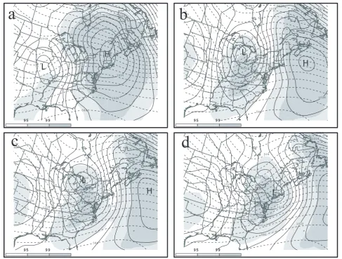
Figure 2.1. Composite of mean sea level pressure, significance of the sea level pressure from climatology, and 500-hPa geopotential height for the Northwestern Low erosion scenario. Mean sea level pressure (solid) every 2 hPa, light shading is 95% significance, dark shading is 99% significance, and 500-hPa geopotential height (dashed) every 4 dam. (a) t-24. (b) t-06 (c) t+00. (d) t+06. centered at demise time (t=0) of CAD………...23 Figure 2.2. As in Fig. 2.1, except for the Cold Frontal Passage erosion scenario………..24 Figure 2.3. As in Fig. 2.1, except for the Coastal Low erosion scenario………...25 Figure 2.4. As in Fig. 2.1, except for the Residual Cold Pool erosion scenario…………26 Figure 2.5. As in Fig. 2.1, except for the Southwestern Low erosion scenario………….27 Figure 3.1 MM5 domain used in simulations of October 2002 case and November 2001

case………..38 Figure 4.1. EDAS analysis of (a) 250-hPa geopotential height (solid, contour interval 12

dam) and isotachs (kts, dashed contours and shaded as in legend at lower left of panel, intervals below 80 kts omitted); (b) 500-hPa geopotential height (solid, contour interval 6 dam), and vorticity (shaded as in legend at lower left of panel, shade interval 4*10-5 s-1); (c) 850-hPa geopotential height (solid, contour interval 3 dam), temperature (dashed, contour interval 4 K), and relative humidity (shaded as in legend at lower left of panel); (d) sea level pressure (solid, contour interval 2-hPa), and 1000-mb temperature (dashed, contour interval 4 K) valid at 0600 UTC 29 Oct 2002………74 Figure 4.2. As in Fig. 4.1, except for 1200 UTC 29 Oct 2002 and 2 m temperature instead

of 1000-mb temperature in panel (d)………...75 Figure 4.3. As in Fig. 4.2, except for 0000 UTC 30 Oct 2002………...76 Figure 4.4. Time scale plot of GSO surface observations from 0000 UTC to 2300 UTC 29 Oct 2002. Top trace is temperature and dewpoint in ºC; Second trace is mean sea level pressure; Third trace is wind barbs and wind speed in knots; Fourth trace is visibility in miles; Bottom trace is sky conditions and weather symbols………77 Figure 4.5. Upper air soundings from Greensboro, NC (GSO) at (a) 1200 UTC 29 Oct

(12)

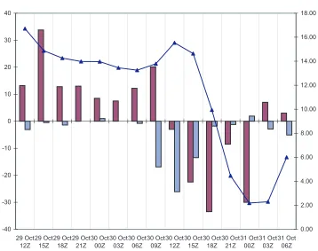
Figure 4.6. Graph depicting relationship between inversion strength and differential potential temperature advection at 850 mb and 1000 mb for GSO between 1200 UTC 29 Oct 2002 and 1200 UTC 31 Oct 2002. Inversion strength is shown by triangles and defined as the potential temperature difference between 850 mb and the surface (K, right y-axis). Potential temperature advection at 850 mb is shown by dark columns (1*10-5 Ks-1, left y-axis). Potential temperature advection at 1000 mb is shown by light columns (1*10-5 Ks-1, left y-axis). Warm advection indicated by positive values and cold

advection indicated by negative values………79

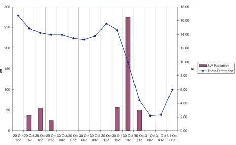
Figure 4.7. Graph depicting relationship between inversion strength at GSO and solar radiation values from High Point, NC between 1200 UTC 29 Oct 2002 and 1200 UTC 31 Oct 2002. Inversion strength defined and shown as in Fig. 4.6. Solar radiation values are shown by columns (Wm-2, left y-axis)…………...80

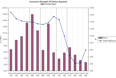
Figure 4.8. Graph depicting relationship between inversion strength and the square of shear at GSO between 1200 UTC 29 Oct 2002 and 1200 UTC 31 Oct 2002. Inversion strength defined and shown as in Fig. 4.6. Shear-squared is shown by columns and defined as ∆U2 + ∆V2 calculated between 850 mb and the surface (1*10-5 s-2, left y-axis)……….81

Figure 4.9. As in Fig. 4.2, except for 1200 UTC 30 Oct 2002………...82

Figure 4.12. As in Fig. 4.4, except for 0000 UTC to 2300 UTC 30 Oct 2002……….85

Figure 4.13. As in Fig. 4.5, except for (a) 1200 UTC 30 Oct 2002 and (b) 0000 UTC 31 Oct 2002. ……….86

Figure 4.14. As in Fig. 4.4, except for 0000 UTC 31 Oct to 2300 UTC 31 Oct 2002…….87

Figure 4.16. EDAS analysis of 1000-mb to 900-mb layer divergence (1*10-5 s-1, shaded as in legend at lower left of panel) and sea level pressure (solid, contour interval 1-hPa) valid at 0000 UTC 31 Oct 2002………….………..89 Figure 4.17. Comparison of NCEP Eta Model forecast sounding (solid bold black lines)

(13)

Figure 4.18. Comparison of surface observations and manually analyzed isotherms with NCEP Eta Model forecast near-surface parameters. (a) Manually analyzed isotherms (solid black lines every 5 °F) and station plots (standard format, temperature and dewpoint in °F and winds in kts) at 1800 UTC 30 Oct 2002. (b) Eta Model forecast showing isotherms (solid, contour interval 5 °F), mean sea level pressure (dashed, contour interval 1 hPa), and winds (barbs in kts) valid at 1800 UTC 30 Oct 2002. (c) as in (a), except at 2100 UTC 30 Oct 2002. (d) as in (b), except valid at 2100 UTC 30 Oct 2002. (e) as in (a), except at 0000 UTC 31 Oct 2002. (f) as in (b), except valid at 0000 UTC 31 Oct 2002………92-94 Figure 4.19. Graph depicting relationship between forecast inversion strength and forecast

differential potential temperature advection at 850 mb and 1000 mb produced by the MM5 control run for GSO between 1200 UTC 29 Oct 2002 and 0600 UTC 31 Oct 2002. Inversion strength is shown by triangles and defined as the potential temperature difference between 850 mb and the 1000 mb (K, right y-axis). Potential temperature advection at 850 mb is shown by dark columns (1*10-5 Ks-1, left y-axis). Potential temperature advection at 1000 mb is shown by light columns (1*10-5 Ks-1, left y-axis). Warm advection indicated by positive values and cold advection indicated by negative values………95 Figure 4.20. Graph depicting relationship between forecast inversion strength and forecast

solar radiation values produced by the MM5 control run for GSO between 1200 UTC 29 Oct 2002 and 0600 UTC 31 Oct 2002. Inversion strength defined and shown as in Fig. 4.18. Solar radiation values are shown by columns (Wm-2, left y-axis)……….96 Figure 4.21. Graph depicting relationship between forecast inversion strength and the

forecast square of shear produced by the MM5 control run for GSO between 1200 UTC 29 Oct 2002 and 0600 UTC 31 Oct 2002. Inversion strength defined and shown as in Fig. 4.18. Shear-squared is shown by columns and defined as ∆U2 + ∆V2 calculated between 850 mb and 1000 mb (1*10-5 s-2, left y-axis)………..97 Figure 4.22. Vertical profile comparison for 1200 UTC 30 Oct 2002: (a) MM5 control run

forecast sounding (solid bold black lines) with GSO rawinsonde data (solid bold gray lines) and (b) NCEP Eta Model forecast sounding (solid bold black lines) with GSO rawinsonde data (solid bold gray lines) showing temperature, dewpoint, and winds (barbs in knots, control run and Eta Model winds bold)……….98 Figure 4.23. Comparison of NCEP Eta Model forecast sounding (bold black lines) with

(14)

Figure 4.24. As in Fig. 4.21, except for 0000 UTC 31 Oct 2002………...100 Figure 4.25. 30-h forecast downward shortwave radiation values for the surface (shaded as in legend at left of panel, shade interval 100 Wm-2) valid at 1800 UTC 30 Oct 2002 for (a) low albedo run, (b) high albedo run, and (c) control run……….……….101 Figure 4.26. Comparison of MM5 forecast upper air soundings valid at 1800 UTC 30 Oct

2002. Control run is dashed with left wind profile, low albedo run is solid bold gray lines with middle wind profile, and high albedo run is solid black bold lines with right wind profile………...102 Figure 4.27. Difference fields of surface potential temperature in K valid at 1800 UTC 30 Oct 2002: (a) Control run values subtracted from low albedo run values and (b) Control run values subtracted from high albedo run values. Solid lines indicate positive differences, while dashed lines indicate negative differences………..103 Figure 4.28. As in Fig. 4.22, except for 1800 UTC 30 Oct 2002………...104 Figure 4.29. Comparison of 30-h forecast PBL height values valid at 1800 UTC 30 Oct

2002 for (a) Blackadar run (shaded as in legend at left of panel, shade interval 100 m), (b) control run (shaded as in legend at left of panel, shade interval 100 m), and (c) control run PBL height values subtracted from Blackadar run PBL height values (solid lines indicate positive differences, dashed lines indicate negative differences)……….105 Figure 4.30. Comparison of 30-h forecast PBL height values valid at 1800 UTC 30 Oct

2002 for (a) Eta M-Y run (shaded as in legend at left of panel, shade interval 100 m), (b) control run (shaded as in legend at left of panel, shade interval 100 m), and (c) control run PBL height values subtracted from Eta M-Y run PBL height values (solid lines indicate positive differences, dashed lines indicate negative differences)………..106 Figure 4.31. Comparison of MM5 forecast upper air soundings valid at 1800 UTC 30 Oct

2002. Control run is dashed with left wind profile, Blackadar run is solid bold gray lines with middle wind profile, and Eta M-Y run is solid black bold lines with right wind profile………...107 Figure 4.32. Difference fields of surface potential temperature in K valid at 1800 UTC 30

(15)

bold gray lines), (b) Blackadar run forecast sounding (solid bold black lines) with GSO rawinsonde data (solid bold gray lines), (c) Eta M-Y run forecast sounding (solid bold black lines) with GSO rawinsonde data (solid bold gray lines), and (d) NCEP Eta Model forecast sounding (solid bold black lines) with GSO rawinsonde data (solid bold gray lines) showing temperature, dewpoint, and winds (barbs in knots, all model forecast winds bold)………109,110 Figure 5.1. Figure 5.1. EDAS analysis of (a) 250-hPa geopotential height (solid, contour

interval 12 dam) and isotachs (kts, dashed contours and shaded as in legend at lower left of panel, intervals below 80 kts omitted); (b) 500-hPa geopotential height (solid, contour interval 6 dam), and vorticity (shaded as in legend at lower left of panel, shade interval 4*10-5 s-1); (c) 850-hPa geopotential height (solid, contour interval 3 dam), temperature (dashed, contour interval 2 K), and relative humidity (shaded as in legend at lower left of panel); (d) sea level pressure (solid, contour interval 2-hPa), and 2-m temperature (dashed, contour interval 4 K) valid at 1200 UTC 23 Nov 2001………..136 Figure 5.2. As in Fig. 5.1, except for 0000 UTC 24 Nov 2001………137 Figure 5.3. As in Fig. 5.1, except for 1200 UTC 24 Nov 2001………138 Figure 5.4. As in Fig. 4.4, except for 0000 UTC to 2300 UTC 24 Nov 2001…………..139 Figure 5.5. As in Fig. 4.5, except for (a) 0000 UTC 24 Nov 2001 and (b) 1200 UTC 24 Nov 2001………140 Figure 5.6. As in Fig. 4.6, except for the period between 1200 UTC 23 Nov 2001 and

1200 UTC 25 Nov 2001……….141 Figure 5.7. Graph depicting relationship between inversion strength at GSO and solar

radiation values from Salisbury, NC between 1200 UTC 23 Nov 2001 and 1200 UTC 25 Nov 2001. Inversion strength defined and shown as in Fig. 4.6. Solar radiation values are shown by columns (Wm-2, left y-axis)………….142 Figure 5.8. As in Fig. 4.8, except for the period between 1200 UTC 23 Nov 2001 and

1200 UTC 25 Nov 2001……….143 Figure 5.9. As in Fig. 5.1, except for 0000 UTC 25 Nov 2001………144 Figure 5.10. Manual surface analysis of coastal front location at 1800 UTC 24 Nov 2001.

Station reports (temperature and dewpoint in °F and winds in kts) and surface fronts are indicated by standard convention………..145 Figure 5.11 EDAS analysis of 1000-mb to 900-mb layer divergence (1*10-5 s-1, shaded as

(16)

1-hPa) valid at (a) 1200 UTC 24 Nov 2001 and (b) 0000 UTC 25 Nov

2001………146

Figure 5.12. As in Fig. 5.1, except for 0600 UTC 25 Nov 2001 and 1000-mb temperature instead of 2 m temperature in panel (d)……….147

Figure 5.13. As in Fig. 4.4, except for 0000 UTC to 2300 UTC 25 Nov 2001………….148

Figure 5.14. As in Fig. 4.5, except for (a) 0000 UTC 25 Nov 2001 and (b) 1200 UTC 25 Nov 2001………149

Figure 5.15. As in Fig. 4.16, except for (a) 1200 UTC 23 Nov 2001, (b) 0000 UTC 24 Nov 2001, (c) 1200 UTC 24 Nov 2001, and (d) 0000 UTC 25 Nov 2001…150, 151 Figure 5.16. As in Fig. 4.17, except (a) at 0000 UTC 25 Nov 2001 and (b) valid at 0000 UTC 25 Nov 2001………..152

Figure 5.17. As in Fig. 4.18, except for the period between 1200 UTC 23 Nov 2001 and 0600 UTC 25 Nov 2001……….153

Figure 5.18. MM5 control run simulation showing isotherms (solid, contour interval 5 °F), mean sea level pressure (dashed, contour interval 1 hPa), and winds (barbs in kts) valid at (a) 1800 UTC 24 Nov 2001 and (b) 0000 UTC 25 Nov 2001………154

Figure 5.21. As in Fig. 4.21, except for 1200 UTC 24 Nov 2001………..157

Figure 6.1. As in Fig. 4.1, except for 0000 UTC 10 Dec 2001………174

Figure 6.4. As in Fig. 4.4, except for 0000 UTC to 2300 UTC 12 Dec 2001…………..177

(17)

Figure 6.7. Graph depicting relationship between inversion strength at GSO and solar radiation values from Siler City, NC between 1200 UTC 12 Dec 2001 and 1200 UTC 14 Dec 2001. Inversion strength defined and shown as in Fig. 4.6.

Solar radiation values are shown by columns (Wm-2, left y-axis)………….180

Figure 6.8. As in Fig. 4.8, except for the period between 1200 UTC 12 Dec 2001 and 1200 UTC 14 Dec 2001……….181

Figure 6.14. As in Fig. 4.5, except for (a) 0000 UTC 14 Dec 2001 and (b) 1200 UTC 14 Dec 2001………187

Figure 6.15. Comparison of NCEP Eta Model forecast sounding (solid bold black lines) from the 1200 UTC 12 Dec 2001 model run with GSO rawinsonde data (solid bold gray lines) for (a) 1200 UTC 12 Dec 2001 and (b) 0000 UTC 13 Dec 2001 showing temperature, dewpoint, and winds (barbs in knots, Eta Model winds bold)……….188

(18)

I. INTRODUCTION

1.1 Motivation

The Appalachian mountain range is known to be a driving force behind many interesting weather phenomena. An example of a common weather pattern induced by the presence of the Appalachian Mountains is cold air damming (CAD). Damming events are initiated when a high pressure system (the “parent high”) moves into the northeastern United States and produces winds that flow nearly perpendicular to the mountain range. A stable atmosphere and the high terrain can block the flow, altering the force balances to produce a northeasterly ageostrophic wind adjacent to the Appalachian ridge. These northeasterly winds advect colder air from the north into the damming region1 and allow for the creation of a vertical cold dome. This lower-tropospheric cold advection influences the development of a capping inversion above the cold dome. The existence of overrunning warm, coastal air may further strengthen the inversion.

Since cold air damming (CAD) events can have significant effects on the weather around the Appalachian region, such as freezing rain and coastal frontogenesis, accurate forecasting is essential. Although most operational forecasting models can capture the onset of a CAD event, they often struggle with CAD erosion by underestimating the duration of sensible effects (Keeter et al., 1995). In order to improve CAD erosion forecasting in

(19)

operational models and inform forecasters of possible model biases, it will be necessary to determine the physical processes of CAD erosion that may cause the largest model error. A better understanding of CAD physical processes will not only benefit those affected by Appalachian cold air damming, but will also be beneficial to the numerous regions impacted by similar weather occurrences worldwide. Smith (1982) described the effects on the flow approaching mountain ranges in Europe, New Zealand, Iceland, and Colorado in which the force balances are disrupted and a pressure difference develops across the terrain. Lackmann and Overland (1989) found similarities in the geostrophic adjustment process between Appalachian cold air damming and gap wind events occurring in Shelikof Strait, Alaska. Additionally, Colle and Mass (1995) examined mountain-parallel cold surges along the Rockies.

1.2 Cold

Air

Damming

Overview

1.2.1 Physical Processes of CAD Initiation

(20)

The Froude number is often used to determine the blocking potential at the windward side of the mountain barrier (Manins and Sawford, 1982), where

NH U

F = (1)

In equation (1), U is the speed of the large-scale, terrain-normal flow, N is the Brunt-Vaisala frequency, and H is the height of the mountain. When squared, this parameter represents the ratio of the kinetic energy of the approaching air mass to the potential energy needed to rise above the barrier (Keeter et al., 1995). Smaller values of the Froude number would indicate that the air mass lacks sufficient inertia and may become blocked by the terrain (Forbes et al., 1987; Bell and Bosart, 1988).

(21)

and maintaining a CAD event. Cloud cover effectively prevents shortwave radiation from warming the surface layers, while the evaporation of falling precipitation further decreases temperatures within the cold dome. Atmospheric stability and surface pressure is thus maintained and/or increased, which leads to stronger blocking of the flow and the initiation or strengthening of cold air damming.

1.2.2 CAD Structure

CAD events initiated and enhanced by strong synoptic forcing are often referred to as classical events (Hartfied et al., 1996; Kramer, 1997; Bailey et al., 2003). Classical CAD events often have a vertical structure characterized by the development of a northeasterly, low-level jet adjacent to the mountain barrier that provides continual cold advection to the damming region (Forbes et al., 1987; Bell and Bosart, 1988). Warm, moist air continues to flow onshore and overruns the cold dome. The vertical differential temperature advection, involving cold advection at low-levels and warm advection aloft, creates an elevated stable inversion (Richwien, 1980; Forbes et al., 1987; Bell and Bosart, 1988). This capping inversion isolates the low-level cold air into the distinct “cold dome” and protects it from becoming mixed with the upper-level flow. The Richardson number, calculated within the inversion layer, can be used to compare the static stability of the inversion to the strength of shear across the inversion (Lackmann and Overland, 1989). For this purpose, the Richardson number is,

( ) ( )

[

2 2

]

z g

Ri

∆ + ∆ ⋅

∆ ⋅ ∆ ⋅ =

(22)

where ∆θ, ∆U, and ∆V are the potential temperature and wind differences calculated across

∆z (Stull, 1988, pp 177). If the calculated value of the Richardson number is greater than 1,

then the layer is considered dynamically stable and laminar. If the Richardson number is less than 0.25, then a laminar layer can become dynamically unstable and turbulent. Although equation (2) is actually the bulk Richardson number, these criteria should still be accurate when examining a capping inversion, since the inversion layer is not exceptionally thick (Stull, 1988, pp. 176-177). A higher Richardson number indicates a stronger capping inversion and a reduced likelihood of turbulent mixing. Therefore, the cold dome would have more adequate protection at its top.

Coastal fronts are another prominent feature of the cold dome structure, often forming along the eastern boundary of the cold dome (Bosart et al., 1972; Riordan, 1990; Keeter et al., 1995). Since there is a distinct temperature gradient above the cold dome similar to an elevated frontal zone, Forbes et al. (1987) described the capping inversion as being a westward extension of the coastal front. As the cold dome erodes toward the end of a cold air damming event, the coastal front may progress inland (Keeter et al., 1995).

1.2.3 CAD Impacts

(23)

from the northeasterly flow, protective cloud cover, and evaporative cooling (Forbes et al., 1987; Bell and Bosart, 1988). Fog and low-level cloudiness are common characteristics of CAD, mainly formed due to the effects of the overrunning warmer, marine air. Conditions such as these reduce visibility and ceiling height. After the high pressure system to the northeast has moved offshore, the low level jet will decrease in strength, and the surface winds become more light or calm. The stable atmosphere and light winds may thus influence air quality in the damming region.

The thermal structure associated with cold air damming can create an environment suitable for dangerous conditions during wintertime events, such as freezing rain and sleet. Predicting precipitation type during a CAD event may be complicated, since the location and extent of the cold dome can often dictate which regions receive frozen precipitation and which regions receive liquid precipitation (Forbes et al., 1987; Keeter et al., 1995). Bell and Bosart (1988) discussed how rain falling down into the cold dome could easily convert into frozen precipitation. Liquid precipitation falling from the warmer, upper levels into the cold dome could change over to sleet and freezing rain. Forbes et al. (1987) performed a case study of a cold air damming event that caused an ice storm in the Appalachian region. Therefore, knowledge of the strength and duration of the cold dome can assist in the warning of possibly hazardous winter precipitation situations.

(24)

damming region from the west or southwest may often redevelop along the coastal front. All of the above CAD impacts and effects will continue until some mechanism or process eventually erodes the cold dome and causes the demise of the event.

1.2.4 Physical Processes Involved in CAD Erosion

Several different processes that may influence cold dome erosion have been identified, but the extent to which each may contribute is not fully understood and is dependent on factors unique to each situation. The dominant processes contributing to erosion may be different for each CAD case, and several processes may be occurring during a single erosion event.

(25)

physical mechanisms that contributed to the evolution and erosion of cold pools in the Columbia Basin of Washington state, which exhibit a similar vertical structure to a CAD cold dome. Model simulation revealed that cold advection aloft weakened the protective capping inversion of the cold pool and was the dominant process influencing erosion for Columbia Basin cold pools. Shear-induced entrainment and mixing at the inversion level, along with cold advection aloft, can be considered physical mechanisms that erode the cold dome from the top down toward the surface.

Cloud cover, a common characteristic of cold air damming events, is another feature that protects the cold dome from dissipation. The clouds prevent shortwave radiation from warming the surface during the daytime (Fritsch et al., 1992). Persistent clouds and fog may even suppress the diurnal temperature cycle, since outgoing longwave radiation would become trapped within the cold dome at night (Zhong et al., 2001). Consequently, the reduction of cloud cover during a CAD event will allow the penetration of radiation into the cold dome and generate a surface heat flux promoting mixing within the low levels. Radiational heating and mixing within the cold dome will weaken the inversion in a similar manner as mixing and entrainment within the inversion level, except the former erodes the cold dome from the surface upwards. In this case, as the cold dome is warmed by shortwave radiation, the ∆θ values will decrease across the capping inversion. Thus, the Richardson number will also decrease, indicating a weaker inversion.

(26)

essentially advect out of the region. The CAD event studied by Bell and Bosart (1988) eroded in this manner, influenced by the presence of a coastal cyclone. The occurrence of this physical process could be identified in successive observations as a lowering of the inversion layer and a decrease in the height of the cold dome. The height tendency equation could be used to examine the raising or lowering of the cold dome and inversion

e w w dt

dH ₌ ₊

, (3)

where w represents the large scale vertical velocity and werepresents entrainment at the

inversion (Lackmann and Overland, 1989). This equation accounts for the effects of divergence by means of the relationship between w and the continuity assumption. In some cases, the inland progression of the coastal front may be an indicator that divergence is occurring within the damming region. If the coastal front represents the eastern boundary of the cold dome, then as the cold wedge narrows in response to the surface divergence, the coastal front may essentially be “pulled” onshore.

1.3 Summary of Objectives

(27)

was overestimated. Keeter et al. (1995) stated that errors could be due to a combination of factors including poor model resolution, limited upper air observations, and inherent model problems when dealing with cloudiness and winds.

As an example, the NCEP Eta model2 often experiences large forecasting errors during CAD erosion. Surface temperatures forecasted by the Eta Model toward the end of an event are often too warm, suggesting that the model erodes the cold dome early. It has been suggested that the NCEP Eta Model may not correctly simulate the interaction between radiation and clouds by allowing too much shortwave radiation to penetrate cloud cover (Ferrier, 2001, personal communication). A study performed by Betts et al. (1997) compared the performance between a 1995 version and a 1996 version of the Eta Model in modeling surface parameters and boundary layer structure during the summer periods of the 1987 FIFE experiment. It was found that both versions of the Eta Model overestimated surface temperatures. Several reasons for the errors were given, such as inaccurate cloud and radiation parameterization schemes, along with insufficient aerosol interactions with shortwave radiation. Yucel et al. (1998) reported similar errors when examining the accuracy of Eta Model-derived surface parameters with observations in Oklahoma, Kansas, and Arizona. Surface temperatures were also overestimated in these cases, especially during daytime cloudiness. Problems with radiation and soil parameterization schemes were considered possible causes of the errors. Although these two studies did not involve cold air damming events, the results may suggest that the Eta Model has inherent difficulties in parameterizing physical processes important in cold dome maintenance and erosion.

(28)

parameterization schemes, CAD initiation seems to be improving. However, these same models still struggle to accurately predict the duration of the event, along with the erosion of the cold dome. A possible explanation is that some of the physical processes involved in cold dome erosion are smaller-scale, which may be more difficult for the model to parameterize. In order to improve forecasts, it is necessary to obtain a better understanding of the physical processes involved in CAD erosion. Zhong et al. (2001) stated a similar necessity for understanding the mechanisms influencing evolution and demise of cold pools in many areas of the United States.

(29)

II. CAD EROSION COMPOSITES

2.1 CAD Detection Algorithm

A CAD detection algorithm was developed in Bailey et al. (2003) that is designed to examine hourly surface data to identify characteristic features of Appalachian cold air damming, thus creating a climatological sample of CAD events for compositing purposes and case study analyses. The algorithm utilizes hourly surface observations, along with NCEP reanalysis grids from the NOAA-CIRES Climate Diagnostics Center. The reanalysis grids have a 2.5° by 2.5° grid spacing, 17 vertical pressure levels, and 6-hour temporal resolution (Kalnay et al., 1996). Both the hourly data and the NCEP reanalysis grids were imported into the General Meteorological Package (GEMPAK).

(30)

In order for the detection algorithm to activate, the calculated Laplacian values for at least one of the three perpendicular lines and the pressure difference values for the parallel line must meet certain criteria: (i) the mountain-normal Laplacian of sea level pressure should generally be negative, (ii) the mountain-normal Laplacian of potential temperature should generally be positive, and (iii) a pressure difference of at least 1.5 hPa must exist along the parallel line between the station located in the middle of the line and one of the endpoint stations.

(31)

2.2 Erosion Scenario Classification

Composite maps of CAD erosion should illustrate common synoptic features representative of the physical processes involved in cold dome erosion. Data provided by the CAD detection algorithm of Bailey et al. (2003) were utilized for the compositing purposes of this study. The CAD events selected for compositing were limited to those identified by the algorithm as having occurred between 1984 and 1995. Additionally, only those categorized as “classical” events were considered. A total of 89 events were selected for analysis.

(32)

1.) Northwestern Low – A surface low pressure system approaches the CAD region from the west to northwest of North Carolina. During the time frame from 24 hours before demise to 6 hours after demise, the low pressure system is centered

between 100°W and 70°W longitude and between 40°N and 60°N latitude. Any associated cold front, determined by the shape of isobars and the gradient of potential temperature, must remain west of the spine of the Appalachian Mountains in North Carolina during CAD erosion.

2.) Cold Frontal Passage – Location of the low pressure system is similar to the Northwestern Low, however, the cold front passes east of the spine of the Appalachian Mountains in North Carolina no later then 6 hours after the demise time.

3.) Coastal Low - A low pressure system is present or develops between 79°W and 60°W longitude and between 40°N and 25°N latitude within the erosion time

period specified above.

4.) Residual Cold Pool – Examination of the NCEP reanalysis grids provides no indication of the existence or development of any prominent synoptic features in the eastern half of the United States. The high pressure system in this scenario may simply become ill-defined and move east to southeast.

5.) Southwestern Low – A low pressure system approaches the CAD region from the south to southwest of North Carolina. Unlike the Coastal Low erosion scenario,

the cyclone is west of 79°W longitude at 24 hours before demise. After this time,

the center of the low system is between 100° W and 60°W longitude and between

(33)

2.3 Erosion Scenario Composites

2.3.1 Compositing Method

As stated in section 1.3, the first research goal is to describe typical synoptic patterns during CAD erosion that may be representative of physical erosion processes. To accomplish this goal, composites of the five erosion scenarios were created using methods similar to those in Colle and Mass (1995), Lackmann et al. (1996), and Bailey et al. (2003). Such composites would facilitate identification of the most prominent patterns associated with each scenario. Each of the 89 CAD events were grouped into one of the five erosion scenario categories according to how closely the event corresponded to the criteria of that scenario. This resulted in 23 Northwestern Low events, 14 Cold Frontal Passage events, 25 Coastal Low events, 23 Residual Cold Pool events, and 4 Southwestern Low events. The reanalysis grids for all events of a certain erosion scenario were then averaged with respect to the demise time to obtain a composite. Averages were calculated every six hours, beginning 24 hours before the demise time and ending 24 hours after the demise time.

2.3.2 Introduction to Composites

(34)

confidence level, according to the two-tailed student-t test (Panofsky and Brier, 1968). Climatological values were determined as in Bailey et al. (2003) using a 12-year monthly average from 1984 to 1995 of the hourly surface data described in section 2.1.

It should be noted that, although composites are ideal for highlighting prominent synoptic features of an erosion scenario, they may not be entirely representative of each individual CAD event. This is especially true as the composite offset time deviates by greater than 24 to 48 hours from the CAD demise time, about which the composites are centered. Since grids were averaged about the demise time, the location and strength of certain features, which may be comparable for that time, could begin to differ considerably as the departure from that time increases. This can result in a somewhat misleading distortion of the features (Lackmann et al., 1996, section 2; Bailey et al., 2003). Therefore, there should be a certain amount of awareness concerning representativeness when examining composites.

2.3.3 Composite Analysis

2.3.3.1 Northwestern Low

(35)

the high pressure system has progressed to the southeast (Fig. 2.1b). Even though the high pressure system is no longer reinforcing the flow into the damming region, CAD effects remain for another six hours. A surface low pressure center is now located over the Great Lakes, northwest of the damming region of North Carolina. Although the resolution is fairly coarse in the composites, a cold front associated with this low system and extending southwest from Illinois to Arkansas can be identified by the surface pressure trough. Figure 2.1c shows the synoptic features for the Northwest Low scenario at demise time. The approaching low system has strengthened, and the cold front has become more clearly defined. However, by the end of the CAD event, the cold front has remained west of the damming region, extending from Indiana to Louisiana. Even at 6 hours after the demise of the event (Fig. 2.1d), the front has still not moved east of the spine of the Appalachians. The failure of the front to reach the damming region suggests that it may not be an important factor in the erosion of the cold dome for this scenario. Instead, the synoptic development indicates that the cold dome may erode due to surface-based divergence toward the lower pressure to the north. Other erosion processes may also be occurring at the same time, including solar mixing within the cold dome and shear-induced mixing at the inversion level.

2.3.3.2 Cold Frontal Passage

(36)

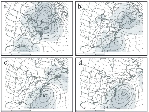
moves eastward, while a surface low develops to the northwest of the North Carolina damming region within the 24 hours before demise. The only notable difference is that the cold front of the Cold Frontal Passage scenario appears oriented slightly more north-south than in the Northwestern Low scenario. It is not until the demise time (Fig. 2.2c) that the most distinguishable difference between the two erosion scenarios appears. The cold front in this scenario has clearly reached the damming region by the end of the CAD event, as it is located from Maryland southward to Georgia. By 6 hours after the demise (Fig. 2.2d), the cold front has progressed entirely east of the spine of the Appalachians. Therefore, the cold front in the Cold Frontal Passage erosion scenario does seem to be influential in the erosion of the cold dome. If cold dome erosion does not begin until after the cold front passes the damming region, then cold advection aloft would be a possible erosion mechanism, acting to

reduce the Richardson number across the protective capping inversion and promote mixing.

However, erosion of the cold dome during a Cold Frontal Passage scenario may be

occurring before the surface cold front appears to progress through the damming region.

Synoptic cold fronts approaching the Appalachian terrain from the west, may undergo

frontal steepening as a result of the mountain barrier (Schumacher et al., 1996; Brennan et

al., 2003). Thus, cold advection aloft, a transition to northwesterly flow, and downsloping

can occur over the damming region, even though the surface front may not appear to have

progressed through the area. In order to further determine the mechanisms involved in CAD

erosion for the Cold Frontal Passage scenario, a detailed case study of a representative

(37)

2.3.3.3 Coastal Low

Figure 2.3 displays the Coastal Low erosion scenario composites. The most prominent synoptic feature at 24 hours and 6 hours before demise (Figs. 2.3a and 2.3b) is the surface low pressure system along the East Coast. Comparison of Figs. 2.1, 2.2, and 2.3 indicates that the high pressure system during this time period does not move as far eastward before demise time as in the Northwestern Low and Cold Frontal Passage scenarios. As the coastal low center develops, the high pressure system appears mainly to weaken and decrease in spatial extent. Between the demise time (Fig. 2.3c) and 6 hours after demise (Fig. 2.3d), the coastal low has deepened. It is the location of this system with respect to the damming

region that impacts the erosion of the cold dome. As demonstrated by Bell and Bosart (1988), the pressure gradient force in the region will be altered due to the lower pressure off the coast. Thus, divergence at the surface will act to reduce the depth of the cold dome. Depending on the exact location of the coastal low, the damming region may remain in cold air throughout CAD erosion. If cold advection begins to occur aloft, while cold advection at the surface is either weaker or nonexistent, then the inversion layer may be weakened in accordance with a reduction in the Richardson number.

2.3.3.4 Residual Cold Pool

(38)

locations at 24 hours before demise (Fig. 2.4a). As time progresses, the high pressure system becomes less organized and eventually moves eastward off of the northeast coast. The deterioration and movement of the high pressure in the CAD region is not strongly influenced by any synoptic feature, which may suggest more of an influence from small-scale processes. The reduction of cloud cover and subsequent penetration of radiational heating and mixing within the cold dome may be a possible factor affecting the erosion in this scenario. However, 11 of the 23 CAD events grouped into the Residual Cold Pool scenario had demise times at or before 8am. This would suggest that radiational heating and mixing would not have been a factor in the erosion of these cases. It is possible that the demise times computed by the CAD detection algorithm were inaccurate for the cases comprising the Residual Cold Pool composite.

2.3.3.5 Southwestern Low

(39)

damming region. Figure 2.5b shows the development of the low system 6 hours before demise. It is now located west of the spine of the Appalachians. The suggestion of a warm front, as indicated by the eastward extending surface trough, has moved over the damming region. At the demise time and 6 hours after the demise (Figs. 2.5c and 2.5d), this surface trough appears to have become an extension of the low center, reaching eastward toward the North Carolina and Virginia coastlines.

2.3.4 Composite Summary

(40)

95 99 1014 1018 1018 1018 1026 H L 528 536 544 552 560 568 576 584 95 99 1012 1012 1016 1016 1020 1024 H L 532 540 548 556 564 572 580 95 99 1012 1012 1016 1016 1020 1020 1020 1024 H L 532 540 548 556 564 572 580 95 99 1012 1012 1016 1016 1020 1020 1024 H L 532 540 548 556 564 572 580

a

b

Figure 2.1. Composite of mean sea level pressure, significance of the sea level pressure from climatology, and 500-hPa geopotential height for the Northwestern Low erosion scenario. Mean sea level pressure (solid) every 2 h-Pa, light shading is 95% significance, dark shading is 99% significance, and 500-hPa geopotential height (dashed) every 4 dam. (a) t-24. (b) t-06 (c) t+00. (d) t+06. centered at demise time (t=0) of CAD.

c

d

(41)

95 99 1014 1014 1018 1018 1026 1030 H L 512 520 528 536 544 552 560 568 576 584 95 99 1010 1010 1014 1014 1014 1018 1018 1022 1026 H L 520 528 536 544 552 560 568 576 584 95 99 1008 1008 1012 1012 1016 1020 1020 1024 H L 520 528 536 544 552 560 568 576 584 95 99 1010 1010 1014 1014 1018 1018 1022 1022 L 524 532 540 548 556 564 572 580

Figure 2.2. As in Fig. 2.1, except for the Cold Frontal Passage erosion scenario.

a

b

d

c

(42)

95 99 1004 1008 1012 1016 1016 1020 1020 1024 1028 H 516 524 532 540 548 556 564 572 580 95 99 1008 1012 1016 1016 1016 1020 1020 H H L 520 528 536 544 552 560 568 576 95 99 1008 1012 1012 1016 1016 1020 1020 H H L 520 528 536 544 552 560 568 576 95 99 1006 1010 1010 1014 1014 1018 1018 1018 H L 528 536 544 552 560 568 576

Figure 2.3. As in Fig. 2.1, except for the Coastal Low erosion scenario.

a

b

c

d

(43)

95 99 1008 1012 1016 1020 1024 1028 1032 H 520 528 536 544 552 560 568 576 95 99 1010 1014 1018 1022 1026 1030H 524 532 540 548 556 564 572 580 95 99 1010 1014 1018 1022 1026 H H 524 532 540 548 556 564 572 580 95 99 1012 1016 1020 1020 1024 H H 524 532 540 548 556 564 572 580

Figure 2.4. As in Fig. 2.1, except for the Residual Cold Pool erosion scenario.

a

b

c

d

(44)

95 99 1000 1004 1008 1008 1012 1012 1016 1016 1020 1020 1020 1024 H L L 536 536 544 552 552 560 568 576 95 99 1000 1004 1004 1008 1008 1012 1012 1016 1016 1020 1020 1024 L 540 540 548 556 564 572 580 95 99 1000 1004 1008 1008 1012 1012 1016 1020 1020 1024 H L 544 552 560 568 576

584 ₉₅ ₉₉

1000 1004 1004 1008 101 2 1016 1020 1020 1020 1024 1024 H L 536 536 544 552 560 568 576

Figure 2.5. As in Fig. 2.1, except for the Southwestern Low erosion scenario.

a

b

c

d

(45)

III. Analysis Tools and Methodology

3.1 Case Selection

Scott Sharp from the National Weather Service office in Raleigh, NC provided

documentation of Appalachian cold air damming events that affected central North Carolina

between 2000 and 2002. From this list, three Appalachian cold air damming events were

selected as case studies. These events were of special interest to National Weather Service

forecasters, as operational forecast models experienced varying degrees of success in

simulating the erosion period. Additionally, the three cases eroded under the influence of

distinctly different synoptic patterns, with two of the three cases representative of CAD

erosion scenarios discussed in Section 2.2.

Consistency with the erosion scenarios was one of the criteria for selection. The first

CAD case occurred between 29 and 31 October 2002. As will be discussed in Chapter 4, this

case is a clear representation of the Coastal Low erosion scenario. The second CAD case

occurred from 23 November to 25 November 2001 and met the criteria for a Northwestern

Low erosion scenario (see Chapter 5). The final CAD case discussed in this study occurred

between 10 and 14 December 2001. Classification into one of the erosion scenarios was

more difficult for this event, as erosion occurred gradually, apparently under the influence of

two separate low-pressure systems (see Chapter 6). The December 2001 event was thus

(46)

The physical processes influencing cold dome erosion, outlined in Section 1.2.4, are

similar for all of the erosion scenarios. Therefore, conducting case study analyses of two of

the five erosion scenarios will still provide insight into these mechanisms. Although it will

be ideal to eventually perform case study analyses of all the erosion scenarios, CAD events

representing the Coastal Low and Northwestern Low scenarios were selected in this study

because the physical processes involved often cause forecast models to produce large errors.

The accurate forecasting of erosion during a Coastal Low and Northwestern Low scenario is

dependent on the ability of the model to simulate small-scale processes, such as differential

thermal advection and shear-induced mixing. In contrast, forecasting models may not

generate such large errors during a Cold Frontal Passage scenario. In these cases, the

accuracy depends more on the model’s depiction of the larger-scale cold front, which

initiates demise much more quickly and dramatically.

3.2 Observational Data

Synoptic and mesoscale features of each case were examined in order to understand

the nature by which the cold dome was eroded. Meteograms at Greensboro, NC (GSO) were

useful for visualizing the changing conditions within the damming region as the CAD event

progressed. It should be noted that station data from GSO were examined frequently in this

study because of the ideal location of this station within the damming region and the

(47)

over the duration of each CAD event. Examination of meteograms allows for the clear

detection of frontal passages and diurnal variations, since the plots provide a timeline of wind

shifts and pressure, dewpoint, and temperature tendencies.

Manual analyses of surface observations were conducted every 3 to 6 hours near the

end of both CAD events. Potential temperature and sea-level pressure fields were contoured

to assess the intensity, placement, and movement of the cold wedge and pressure ridge within

the CAD region. Gradients of potential temperature were useful in detecting the presence of

any approaching fronts.

It is with some caution that sea-level pressure data are utilized when studying the

development of the high-pressure ridge associated with cold air damming. In areas where the

distance between sea level and the ground surface is greater than 1000m, certain assumptions

concerning the temperature lapse rate beneath the surface must be made when reducing

station pressure to sea level. Pielke and Cram (1987) noted that inaccuracies in these

calculations often result in overestimated pressure values for areas in the basin east of the

Rocky Mountains when cold air is dammed within. However, at locations where the layer

between sea level and the surface is less than 1000m, empirical corrections may not be

necessary (Wallace and Hobbs, 1977, pp 60). The CAD pressure ridge and CAD sensible

weather often extends to areas east of the Appalachian terrain, where the elevation is below

1000m. Thus, it is less likely that the high-pressure ridge is only a result of inaccuracies in

sea-level pressure reduction. Alternative methods have also been used to examine the CAD

pressure ridge, such as altimeter setting by Bell and Bosart (1988).

As a supplement to surface observation reports, radar mosaic imagery at 2km

(48)

Precipitation falling into an unsaturated cold dome could act to maintain and reinforce the

event (see Section 1.2.1).

As discussed in Section 1.2.4, changes in the strength of the protective capping

inversion are a measure of the strength of the cold dome. Thus, variations in the vertical

temperature structure of the atmosphere at a location within the damming region may reveal

the physical processes influencing erosion. Upper air soundings at GSO were obtained at 00

UTC and 12 UTC for the duration of each CAD case study event. Certain parameters were

calculated from the upper air data that provided insight into the nature of the cold dome

erosion. The difference in potential temperature between the surface and 850 hPa was

calculated to indicate the strength of the capping inversion. For both CAD cases, the lowest

inversion layer did not often extend above the 850-hPa level, so this level was considered

representative of the top of the inversion. The square of wind shear over the same layer,

from the surface to 850 hPa, was also calculated using wind component and height values

from the GSO soundings

2 2

     

∆ ∆ +

     

∆ ∆

z v z

u

, (5)

where ∆z is the height at the surface subtracted from the height at 850 hPa. This parameter

was used to indicate the likelihood of shear-induced mixing within the inversion.

Given that incoming shortwave radiation is a possible erosion mechanism (see

Section 1.2.4), solar radiation data were obtained from locations within the damming region.

These data were obtained from the Agricultural Weather Network (Agnet) maintained by the

State Climate Office of North Carolina and the North Carolina Agricultural Research Service

(49)

High Point data were not available prior to 2002, data from the Siler City Airport station in

Siler City, NC were used in the analysis of the December 2001 case, as it is the nearest

station to High Point and Greensboro. This station was missing data during the November

2001 case, so data from the Piedmont Research Station in Salisbury, NC were used. These

stations were selected because they are located in the region where the cold wedge and

pressure ridge often extend and where the sensible effects of CAD are evident. Observed

solar radiation values will be compared to model radiation values in Chapters 4, 5, and 6.

GOES-8 satellite imagery at 4-km was also examined to determine the extent to which solar

radiation may have been able to penetrate to the surface.

3.3 NCEP Eta Model

3.3.1 EDAS Analyses

Along with raw observational data, gridded analyses from the National Centers for

Environmental Prediction (NCEP) Eta Data Assimilation System (EDAS) were examined for

the three cold air damming case studies. The EDAS initializes the NCEP Eta Model as

described in Rogers et al. (1995). The NCEP Eta Model is an operational mesoscale model

that utilizes the eta vertical coordinate to simulate terrain (Mesinger, 1984). At the time of

the case studies, the model was run with a horizontal resolution of 12km and 60 vertical

levels (Rogers et al., 2001). EDAS and Eta Model data sets used in this study had been

interpolated to a grid with a 40-km (Eta 212) or 80-km (Eta 211) horizontal grid spacing and

(50)

The EDAS involves the intermittent update of analyses with the previous 3-hour Eta

Model forecasts. The frequent updates allow more observational data to be incorporated into

the model and improve accuracy. A critical point when examining EDAS analyses is that the

data from previous short-term Eta Model forecasts are assumed to be reliable when

incorporated into the analyses. Before interpolation, comparisons made between the

forecasts and observations can result in small corrections to the forecasts. However, the

system may still allow short-term forecast inaccuracies to persist into the analyses. In

consideration of this issue, evaluation of EDAS grids should be conducted simultaneously

with evaluation of observations and data from other sources.

EDAS analyses were used in the cases studies to supplement basic surface and

upper-air observational data. One of the benefits of these analyses is that they incorporate

additional observations from a multitude of sources that may be otherwise difficult or

time-consuming to obtain and manually analyze, such as data from satellites, radar, wind profilers

and the ACARS network (COMET, 2003). Accordingly, EDAS analyses were used to

evaluate atmospheric conditions at a higher vertical resolution than what is attainable from

manually analyzing surface and upper air observations. The EDAS analyses were also used

to compute parameters not available from basic observational reports and which would

otherwise involve numerous calculations to obtain, such as differential thermal advection.

Contoured maps of sea-level pressure and 500-hPa height fields were obtained from

EDAS analyses at 00, 06, 12, and 18 UTC. These plots were used to assess the evolution of

synoptic features indicative of the erosion scenario for each case, such as the coastal low

system in the October 2002 event. As with the upper air sounding data, certain parameters

(51)

each case. Contoured maps of potential temperature advection at 850 hPa and 1000 hPa were

plotted and analyzed in order to study the effects of differential advection on the capping

inversion.

3.3.2 Eta Model Forecasts

Along with an overview of each event, the accuracy of NCEP Eta Model forecasts

valid during the erosion of each case study was evaluated. The NCEP Eta model is widely

used as an operational forecasting tool, therefore an understanding of common model errors

and biases is important. Furthermore, clarifying the nature of Eta Model errors should also

provide insight into which model sensitivity tests would be most relevant.

To perform this evaluation, Eta Model forecasts valid during the erosion of each

event were compared to EDAS analyses and observations. Model-forecasted sea level

pressure and 500-hPa height fields were obtained for comparison to analyses. Model 10m

winds and 2m temperature fields were compared with surface observations. Additionally,

model-forecasted upper air profiles for Greensboro, NC (GSO) were obtained for comparison

to observed GSO upper air soundings. Evaluation will focus on the depiction of synoptic

scale features such as surface low-pressure centers and frontal systems, as well as local

features such as moisture and wind profiles and the vertical temperature structure.

Comparisons between model forecasts and observations of these features should clarify

whether the same simulated physical processes are eroding the cold dome in the model as in

(52)

3.4 PSU/NCAR MM5 Model

3.4.1 Model Description

As the second objective of this research (see Section 1.3), the fifth generation

Pennsylvania State University-National Center for Atmospheric Research Mesoscale Model

(MM5) Version 3.5 will be used to conduct sensitivity tests of the CAD cases. Results of

these tests should elucidate the roles of various physical processes in the erosion of CAD.

The PSU/NCAR MM5 Model is a non-hydrostatic mesoscale model that utilizes the sigma

vertical coordinate system (Grell et. al, 1994; Dudhia et al., 2000). The MM5 is ideal for this

study because it allows for a high level of user interaction.

Several pre-processing programs are involved in the preparation of an MM5

simulation. When used in conjunction with a land-surface model, the program TERRAIN

sets up the horizontal dimensions of the user-defined model domain and interpolates

information regarding elevation, land use, and soil temperature onto this domain (Dudhia et

al., 2000). Gridder, a program created by the University of Utah Department of

Meteorology, provides the initialization of the MM5 Model. It allows the user to specify

NCEP EDAS analyses as initial and lateral boundary conditions. The initial conditions

incorporated into the MM5 Model will have data on the vertical pressure coordinate system.

The final pre-processing program, INTERPF, transforms this data onto the sigma coordinate

(53)

3.4.2 Model Simulations

A basic model simulation was conducted as a control run for the October 2002 and

November 2001 case studies. This control run simulation was used to facilitate the study of

important erosion mechanisms and the evaluation of errors in modeling erosion. Certain

aspects of the model design were consistent among the control run and all sensitivity test

simulations. Each model run utilized a single domain with 36-km horizontal grid spacing

and 61 x 55 grid points. The domain area was selected to best capture the influence of

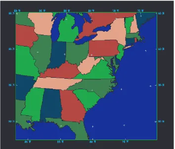
synoptic and mesoscale features on CAD erosion. Figure 3.1 displays the location of the

domain. All model simulations included 45 vertical sigma levels, including the surface. The

MM5 was initialized using NCEP EDAS analyses interpolated to a 40-km grid spacing with

28 vertical pressure levels, including the surface, at 25-hPa intervals up to 600 hPa and

50-hPa intervals up to 100 50-hPa. Boundary conditions for the MM5 were also obtained from the

EDAS analyses and updated every six hours.

Results obtained from the MM5 simulations should be applicable to operational

forecasting issues. Therefore, parameterization schemes were selected based on their

resemblance to schemes used in operational models. The NCEP Eta Model uses a version of

the Betts-Miller convective parameterization scheme, thus the MM5 simulations also used

this scheme (Betts, 1986; Betts and Miller, 1986). Because CAD events are not usually

associated with convection, sensitivity to the convective parameterization scheme is not

likely to be significant. The MRF-PBL scheme (Hong and Pan, 1996) was selected for the

MM5 control runs, mainly for its compatibility with the OSU Land Surface Model (hereafter

(54)

improve simulation of the important physical processes occurring near the surface during

cold air damming events. Chen and Dudhia (2001) also combined the MRF-PBL and

OSU-LSM for MM5 experiments designed to test the effectiveness of the land surface model.

Based on the concept of non-local vertical diffusion, the MRF-PBL scheme is ideal for

well-mixed and unstable boundary layers (Hong and Pan, 1996). It should be noted that this

design, which makes the MRF-PBL suitable for unstable conditions, may also cause the

scheme to overestimate the depth of turbulent mixing within the boundary layer. Braun and

Tao (2000) saw evidence of this occurrence in their study concerning the sensitivity of the

MM5 Model to PBL schemes during hurricane forecasting. Microphysics were

parameterized using the Dudhia Simple Ice scheme (Dudhia, 1989), and radiation was

parameterized using the Cloud-Radiation scheme (Dudhia, 1989). Parameterization schemes

for convection, microphysics, and radiation remained unchanged for the control runs as well

as the sensitivity tests.

Parameters indicative of the nature of cold dome erosion were computed from the

MM5 co