Bayesian Analysis of Circular Data Using Wrapped Distributions

(1)

RAVINDRAN, PALANIKUMAR. Bayesian Analysis of Circular Data Using Wrapped

Dis-tributions. (Under the direction of Associate Professor Sujit K. Ghosh).

Circular data arise in a number of different areas such as geological,

meteorolog-ical, biological and industrial sciences. We cannot use standard statistical techniques to

model circular data, due to the circular geometry of the sample space. One of the

com-mon methods used to analyze such data is the wrapping approach. Using the wrapping

approach, we assume that, by wrapping a probability distribution from the real line onto

the circle, we obtain the probability distribution for circular data. This approach creates

a vast class of probability distributions that are flexible to account for different features of

circular data. However, the likelihood-based inference for such distributions can be very

complicated and computationally intensive. The EM algorithm used to compute the MLE is

feasible, but is computationally unsatisfactory. Instead, we use Markov Chain Monte Carlo

(MCMC) methods with a data augmentation step, to overcome such computational

difficul-ties. Given a probability distribution on the circle, we assume that the original distribution

was distributed on the real line, and then wrapped onto the circle. If we can unwrap the

distribution off the circle and obtain a distribution on the real line, then the standard

sta-tistical techniques for data on the real line can be used. Our proposed methods are flexible

and computationally efficient to fit a wide class of wrapped distributions. Furthermore, we

can easily compute the usual summary statistics. We present extensive simulation studies

to validate the performance of our method. We apply our method to several real data sets

(2)

frequentist coverage probability. We extend our method to the regression model. As an

example, we analyze the association between ozone data and wind direction. A major

con-tribution of this dissertation is to illustrate a technique to interpret the circular regression

coefficients in terms of the linear regression model setup. Regression diagnostics can be

developed after augmenting wrapping numbers to the circular data (refer Section 3.5). We

extend our method to fit time-correlated data. We can compute other statistics such as

cir-cular autocorrelation functions and their standard errors very easily. We use the Wrapped

Normal model to analyze the hourly wind directions, which is an example of the time series

(3)

by

Palanikumar Ravindran

A dissertation submitted to the Graduate Faculty of North Carolina State University

in partial satisfaction of the requirements for the Degree of

Doctor of Philosophy

Department of Statistics

Raleigh 2002

Approved By:

Dr. Peter Bloomfield Dr. Sastry Pantula

Dr. Sujit K. Ghosh Dr. John Monahan

(4)

(5)

Biography

Palanikumar Ravindran was born in Virudhunagar, India, to parents Ravindran Palanichamy

and Rajakumari Ravindran on Oct 25, 1976. He entered Indian Statistical Institute,

Cal-cutta, India in 1994 and received a B.S. and M.S. in Statistics in 1997 and 1999, respectively.

Since August 1999, he has studied for the doctoral degree in the Department of Statistics

(6)

Acknowledgements

I would like to express my deepest gratitude and appreciation to my advisor Dr. Sujit

Ghosh for his guidance, encouragement and support throughout my dissertation research.

I would also like to thank the other committee members, Dr. John Monahan, Dr. Peter

Bloomfield, Dr. Sastry Pantula and Dr. Gene Brothers for their careful reading of this

manuscript and their helpful comments.

It has been a very pleasant experience to study in this department. I would like

to convey my gratitude to the faculty and staff for their help and assistance. Thanks to my

fellow students for their help and support. I would also like to thank Dr. Kaushik Ghosh,

(7)

List of Figures

1.1 Circular histogram plot of the turtle data. Solid line indicates the circular

mean and dashed line indicates the linear mean. . . 4

2.1 Probability plot of{Hk}forµ parameter of WN model . . . 33

2.2 Plot of ρfor the bimodal distribution . . . 35

2.3 Plot of the bimodal density forρ= 0.087 . . . 36

2.4 Plot of the bimodal density forρ= 0.087 on the circle . . . 36

2.5 Circular plot of the Jander’s Ant data . . . 39

2.6 Trace plots while fitting WC to Ant data . . . 41

2.7 Posterior density ofµ while fitting WC to Ant data . . . 42

2.8 Plot of wind directions in the ozone data. . . 43

3.1 Joint data plot of the ozone data. The ozone concentrations are plotted as distances from the center. . . 46

3.2 Plot of the original values. . . 63

3.3 Regression Plot of the sample and fitted values. . . 63

3.4 Plot of wind directions in the ozone data. . . 65

3.5 Trace plots while fitting WN to the Ozone data . . . 68

3.6 Regression Plot of the fitted values. . . 69

3.7 Plot of the residuals. . . 69

4.1 Plot of the median direction of face cleat collected at Wallsend Boreland Colliery, NSW in Australia. . . 72

4.2 Relation between circular autocorrelation function and autocorrelation function 77 4.3 Plot of hourly wind directions collected over three days. . . 80

4.4 Trace plots while fitting WARN(1) to Wind direction data using time series model . . . 81

(10)

List of Tables

2.1 Fitting WN to WN distribution using different priors . . . 24

2.2 Fitting WC to WC distribution using different priors . . . 25

2.3 Fitting WDE to WDE distribution using different priors . . . 25

2.4 Fitting WN, WC and WDE to WN distribution with ρ∼Beta(0.5,0.5) . . 27

2.5 Fitting WN, WC and WDE to WC distribution with ρ∼Beta(0.5,0.5) . . 28

2.6 Fitting WN, WC and WDE to WDE distribution withρ∼Beta(0.5,0.5) . 29 2.7 Fitting WN, WC and WDE to VM data withρ∼Beta(0.5,0.5) . . . 31

2.8 Fitting WEV to WEV distribution . . . 37

2.9 Fitting WB to WB distribution . . . 37

2.10 Fitting WN, WC and WDE to the Ant data set withρ∼Beta(0.5,0.5) . . 40

2.11 Fitting WN, WC and WDE to the Ozone data set withρ∼Beta(0.5,0.5) . 44 3.1 Regressing WN model to WN data . . . 54

3.2 Regressing WC model to WC data . . . 55

3.3 Regressing WDE model to WDE data . . . 56

3.4 Regressing WN, WC and WDE models to WN data withβ1 = 1.5 . . . 58

3.5 Regressing WN, WC and WDE models to WC data withβ1= 1.5 . . . 59

3.6 Regressing WN, WC and WDE models to WDE data with β1= 1.5 . . . . 60

3.7 Regressing WN, WC and WDE models to VM data withβ1= 1.5 . . . 61

3.8 Regressing WN, WC and WDE models to the Ozone data set with ρ ∼ Beta(0.5,0.5) . . . 67

4.1 Regressing WARN(1) model to WARN(1) data . . . 79

(11)

Chapter 1

Introduction to Circular Data

Circular data arise from a number of sources in our daily lives, where we consider

the circle to be the sample space. Some common examples are the migration paths of birds

and animals, wind directions, ocean current directions and patients’ arrival times in an

emergency ward of a hospital. Many examples of circular data are found in various scientific

fields such as earth sciences, meteorology, biology, physics, psychology and medicine. To

motivate the use of circular data, we present a brief description of some examples from

these fields.

1.1 Some real life applications of circular data

The study of earth sciences yields two good examples of circular data - The

orien-tation of cross-bedding structures and the orienorien-tation of the long axis of unbroken sediment

particles. Orientation of the cross-bedding structures gives us information about the

(12)

has proved to be useful in the study of glacial deposits and direction of ice movement.

Pincus (1953) presents several such examples.

In meteorology, wind directions and ocean current directions give rise to circular

data. Johnson and Wehrly (1977) did some analysis of wind directions. Seasonal weather

changes such as the propensity for rainfall during the monsoon season is another example

of circular data.

In the field of physics, before the discovery of isotopes, Von Mises (1918) proposed

testing the hypothesis that atomic weights are integers subject to error. He converted the

fractional parts of the atomic weights to angles. He regarded these angles as a random

sample from a circular distribution with mean zero and tested for uniformity. He also

introduced Von Mises distribution, a popular distribution on the circle. In another study,

Rayleigh (1919) worked with a representation of sound waves. He was interested in the

resultant of unit vectors and its distribution. He considered the unit vectors as points on

the circle.

In psychology, circular data arises from experiments to study the behavior of the

human mind. Consider the simulated tests of zero gravity. Scuba divers were required to

turn somersault and reorient themselves to the vertical under various circumstances (for

example, blindfolded or looking through a translucent faceplate, see Ross et al., 1969).

The angles from the vertical were measured and analyzed. Circular data also occur in the

studies of mental maps, which are used to represent surroundings. Individual subjects were

led past a series of sites. They were asked at each site to point to the direction, and guess

(13)

In medicine, circular data arises as the time of onset of a particular disease at

various times of the year (Lee, 1962). Another example is circadian rhythms, which is the

time of adverse event occurrences throughout the day. Circadian rhythms are analyzed

because it has been found that adverse events (for example, deaths, myocardial infarctions)

do not occur randomly throughout the day but cluster at certain points in the day (Proschan

and Follmann, 1997).

A very good source of circular data is the field of biology. Migration path of birds

and animals has been the subject of many studies. The objective of these studies is to

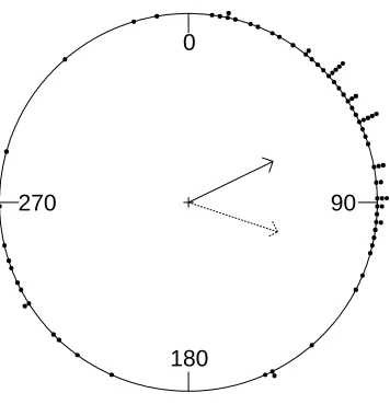
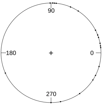
ascertain whether the direction of migration is uniform. An example of the migration of

turtles is given in Figure 1.1. In the figure, we present the circular histogram plot of the

data collected by Dr. E. Gould from John Hopkins University School of Hygiene and first

cited by Stephens (1969). The data represents the directions taken by the sea turtles after

laying their eggs. The predominant direction is 64◦, which is the direction the turtles took

to return to the sea (Fraser, 1979).

Standard statistical techniques cannot be used to analyze circular data. This is due

to the circular geometry of the sample space. For example, the sample mean of a data set

on the circle is not the usual sample mean. Let y1, y2, . . . , yn be independent observations

on the unit circle, such that 0 ≤ yj < 2π, j = 1,2, . . . , n. The mean direction ¯y is not

given by the usual definition, 1_nPn_j₌₁yj. This is illustrated in Figure 1.1, where the dashed

arrow is the direction represented by _n1Pn_j₌₁yj and the solid arrow represents the mean

(14)

0

180

270 90

Figure 1.1: Circular histogram plot of the turtle data. Solid line indicates the circular mean and dashed line indicates the linear mean.

We considerC= _n1 Pn_j₌₁cosyj and S= 1_n

Pn

i=1sinyj and define,

¯

y=

      

arctan(S

C) , C≥0

arctan(S

C) +π , C <0,

where arctan takes values in [−π₂,π₂]. In general, the pth theoretical moment of a circular

distribution is defined as E(eipY) = αp +iβp, for p = 1,2, . . .. The mean direction is

given by µ = arctan(β1/α1) and the mean resultant is defined as ρ = pα21+β12, so that

E(eiY) =ρeiµ. In most applications it is of interest to estimate the location parameterµand

the scale parameter ρ. Nonparametric methods are suitable for this purpose. However, for

the prediction problem, it would be of interest to develop parametric models. In addition,

we exemplify that the class of parametric models that we develop is robust against erroneous

models.

(15)

an emphasis on the wrapping approach. In this dissertation, we use the wrapping method

to generate a flexible class of circular distributions. In chapter 2, we discuss classical and

Bayesian methods to obtain estimates of the parameters of wrapped circular distributions.

As the Bayesian methods have the advantage of obtaining a finite sample estimate of the

variability (for example, s.e. of the estimates), we propose a data augmentation method for

parameter estimation. In Section 2.2, we present the data augmentation method to obtain

the posterior distribution of the parameters of several wrapped distributions. In Section 2.3,

we describe the possible methods for model selection. In Section 2.4, we present extensive

simulation studies to validate the frequentist performance of our method. In Section 2.6,

we discuss the Wrapped Extreme Value and bimodal distributions. In Section 2.7.1, we

apply our method to a real data set on the movement of ants. In chapter 3, we develop

some models for regression where the response variable can be circular or linear. In Section

3.3, we present the extension of the data augmentation method proposed in Section 2.2 for

regression to obtain the posterior distribution of the regression coefficients based on several

wrapped distributions. In Section 3.4, we present extensive simulation studies to validate

the performance of our method for regression. In Section 3.6, we fit a linear regression

model to explore the relation between ozone concentration and wind direction. In Section

4.3, we illustrate how the data augmentation method used for regression in Section 3.3 can

be easily extended for time series. Simulation studies with the Wrapped Normal density

for the time series model is given in Section 4.4. In Section 4.5, we analyze hourly wind

directions, which is an example of time series data. We use the Wrapped Normal model for

(16)

1.2 Statistical Approaches to model circular data

Many methods and statistical techniques have been developed to analyze and

understand circular data (see Mardia and Jupp, 1999). The popular approaches have been

theembeddingapproach, intrinsicapproach andwrapping approach. A brief description of

each of the approaches is given below.

1.2.1 The Embedding Approach

In the embedding approach, the sample space (for example, the unit circle) is

considered as a part of a larger space (for example, 2-dimensional plane). A common

example is the representation of the points of the unit circle by unit complex numbers.

There are many advantages of the embedding approach. Considering the points on the unit

circle, as a vectorx= (cosy,siny)T in the plane enables the use of the traditional definition

of expectations that is used for data in the Euclidean space. For instance, definition of the

mean µof a random variable y, defined on the unit circle is given by

kE[(cosy,siny)T]k−1 E[(cosy,siny)T] = (cosµ,sinµ)T.

Several bivariate distributions on the Euclidean space can be embedded to produce

distribution on the circle. For instance, the Projected Normal distribution is an example

of the embedding approach. In the embedding approach, we start with the larger sample

space (for example, 2-dimensional plane) and obtain the projection of this space into a

smaller sample space. For example, if X has the Bivariate Normal distribution N2(µ,Σ),

then k X k−1 X is said to have the Projected Normal distribution, P N2(µ,Σ). This is

(17)

distri-bution and the resulting marginal distridistri-bution for wind direction is the Projected Normal

distribution. The density ofP N2(µ,Σ) has been derived by Mardia (1972). The Projected

Normal distribution can be extended to p-dimensions, where the distributions on <p are

projected ontoSp−1, the unit sphere in <p. The density of the Projected Normal

distribu-tion, P Np(µ,Σ) has been derived by Bingham (Watson, 1983, pp. 226-231) and a simpler

form was derived by Pukkila & Rao (1988). However, in general, the densities obtained by

embedding a generic distribution on<p ontoSp−1, can turn out to be very complicated and

hence obtaining the likelihood-based inference can be extremely challenging. Therefore,

most of the literature is focused on developing statistical methods for the Projected Normal

distributions only, which is a significant limitation of the embedding approach.

There are some techniques for parameter estimation in the embedding approach.

Spherically projected multivariate linear (SPML) model using P N2(µ,Σ) distribution was

suggested by Presnell, Morrison and Littel (1998). They considered circular data as data

sampled from a plane and projected onto the circle. They assumed that the distance

from the center for each data point, |yi| was missing and used EM algorithm to estimate

it. Embedding technique is also very useful to perform analysis of variance (ANOVA) for

circular data. ANOVA for circular data was proposed by Harrison, Kanji and Gadsen (1986)

and Harrison and Kanji (1988). We do not pursue any analysis based on the embedding

approach in this research work, as the analysis becomes analytically and computationally

(18)

1.2.2 Intrinsic Approach

In the intrinsic approach for circular data, circle is used as the sample space. The

directions (angles) are represented as points on the circle. In intrinsic approach, probability

distributions are defined on the circle directly (for example, Von Mises and Cardioid

dis-tributions). Von Mises distribution is one of the most popular distributions that come out

of this approach. The probability density function of the Von Mises distribution is given

by fV M(y) = ₂_πI1₀₍_κ₎eκcos(y−µ), where I0 denotes the modified Bessel function of the first

kind and order 0. I0 is defined by I0(κ) = ₂1_π R₀2πeκcos(y)dy. Von Mises distribution has

been studied extensively. Mardia and Jupp (1999) give references for the genesis of the

Von Mises distribution on the circle, which is analogous to the Normal distribution on the

real line. Let y={y1, y2, y3, . . . , yn},0≤yi <2π, i= 1. . . nbe a random sample from Von

Mises distribution with location parameter µ and scale parameter κ. Define C, S and R

as C = Pn_i₌₁cosyi, S =

Pn

i=1sinyi and R2 = C2 +S2. C = Rcos ¯y and S = Rsin ¯y,

where ¯y is the mean as defined earlier (in Section 1.1). Mardia and Jupp (1999) provide

the joint distribution of ¯y andR. They give the marginal densities ofR,C andS using the

results given by Greenwood and Durand (1955). Mardia (1972) showed that the conditional

distribution of ¯y givenR is Von Mises distribution with location parameterµand scale

pa-rameter κR. Mardia and Jupp (1999) give results and references on several extensions of

these results to multi-sample Von Mises populations. The asymptotic distributions of these

statistics, as the sample size goes to infinity, are also available.

From a Bayesian perspective, the conjugate prior for the Von Mises distribution

(19)

full Bayesian analysis involving Von Mises distribution, where both the parameters are

assumed to be unknown, and used its conjugate prior proposed by Guttorp and Lockhart.

They proposed MCMC methods to simulate samples from the posterior distribution.

Mardia and Jupp (1999) describe the maximum likelihood estimates for the Von

Mises distribution and give references and results for their large-sample asymptotic

prop-erties. They also provide a good overview of the various single-sample, two-sample and

multi-sample hypothesis tests for the Von Mises distribution.

One of the main drawbacks of the intrinsic approach is that there are not many

distributions available other than the Von Mises distribution and mixture of Von Mises

distributions. Again, due to this limitation, we do not pursue any analysis using this

approach. We use wrapping approach (see next section) and illustrate how a flexible class

of models can be obtained.

1.2.3 Wrapping Approach

In the wrapping approach, given a known distribution on the real line, we wrap

it around the circumference of the circle with unit radius. Technically this implies that if

U is a random variable on the real line, then the corresponding random variable Y on the

circle is given by Y =U(mod 2π). Equivalently, the wrapped version ofU is obtained by

defining Y =U−2π£₂U_π¤, where [u] = largest integer≤u. Let the distribution function of

U on the real line be denoted byF. The distribution function ofY denoted by Fw can be

obtained as,

Fw(y) = Pr(Y ≤y) =

∞

X

k=−∞

(20)

This implies that if the densityf of U exists, then the wrapped density fw is given by

fw(y) =

∞

X

k=−∞

f(y+ 2πk),0≤y <2π.

An excellent overview of the properties of the wrapped distributions can be found

in Mardia and Jupp (1999). One of the properties of the wrapped distributions is that the

characteristic function (c.f.) ofU is same as the c.f. of theY. Thus, from the information

about U, we can obtain the information about Y. More importantly, if the c.f. of U is

integrable, then it can been shown that the density ofY,fw(y) can be represented as,

fw(y) = ₂1_π



1 + 2

∞

X

p=1

(αpcospy+βpsinpy)

 ,

where E(eipY) = E(eipU) = αp +iβp This result on the unit circle is analogous to the

inversion theorem for continuous random variables on the real line. However, in most cases

the above series cannot be written in closed form except in a few cases such as the Cauchy

distribution. One of the most popular wrapped distributions is the Wrapped Cauchy

dis-tribution, introduced by L´evy (1939). This is because the density of the Wrapped Cauchy

distribution has a closed form representation. The density of the Wrapped Cauchy

dis-tribution is given by P∞_k₌_−∞_πσ1

·

1 +

³

y+2πk−µ σ

´2¸−1

, where µ is the location parameter

and σ is the scale parameter. Using the inversion theorem, this can be represented as

1

2π{1 + 2

P_∞

1 (ρpcosp(y−µ))}, where ρ = e−σ. Considering this density as the real part

of the geometric series P∞₁ ρpe−ip(y−µ), simplifies it to ₂1_π₁₊_ρ₂₋1₂−_ρρ_cos(2 _y₋_µ₎. Kent and Tyler

(1988) and Mardia (1972) have shown the relation between the Wrapped Cauchy

distribu-tion and the Projected Normal distribudistribu-tion. Mardia and Jupp (1999) describe the wrapped

(21)

This is a larger family of distributions containing the Wrapped Cauchy distribution (α= 1)

and the Wrapped Normal distribution (α= 2).

It follows that a rich class of distributions on the circle can be obtained using the

wrapping technique because we can wrap any known distribution on the real line onto the

circle. Also, by wrapping a symmetric unimodal density, it is possible to obtain a bimodal

density on the circle. An example is the Wrapped Beta distribution. We discuss this in

Section 2.6. The main difficulty in working with the wrapping approach has been that, in

most cases, the form of the densities and distribution functions are large sums, and cannot be

simplified as closed forms. Due to this complexity, maximum likelihood techniques for point

estimation and hypothesis testing cannot be easily implemented. The main contribution of

this dissertation is to present a general approach to obtain parameter estimates of a wide

class of wrapped distributions. The next paragraph outlines our approach.

For a given probability distribution on the circle, we make assumptions that the

original circular distribution was distributed on a line and was wrapped onto the circle.

Therefore if we can unwrapthe distribution on the circle and obtain a distribution on the

real line, we can use all the standard statistical techniques for data on the real line. We

propose to perform this using the data augmentation approach. We use Bayesian methods,

so that we can easily obtain parameter uncertainty estimates based on the finite sample.

In many practical problems (as discussed in Section 1.1), the sample sizes are usually small

(22)

Chapter 2

Parameter Estimation for Wrapped

Distributions

In this chapter, we consider parameter estimation for several wrapped

distribu-tions. We concentrate on symmetric unimodal and bimodal densities.

2.1 Previous Work

It was shown by Kent and Tyler (1988) that the maximum likelihood estimate for

the Wrapped Cauchy distribution exists and is unique for samples of size greater than two.

They also gave a simple iterative algorithm, which would always converge to the maximum

likelihood estimate (MLE). Calculating the MLE for the Wrapped Cauchy distribution

is possible because the density has a closed form representation. In general, wrapped

distributions do not have closed form densities and consequently, computing the MLE is

(23)

A different approach for fitting wrapped distributions was given by Fisher and

Lee (1994) who used the Expectation Maximization (EM) algorithm techniques to obtain

parameter estimates from the Wrapped Normal distribution. However, the E-step involves

ratio of large infinite sums, which needs to be approximated at each step. This makes the

algorithm computationally inefficient. In addition, the standard errors of the MLEs have to

be evaluated based on large-sample theory. We propose an alternative method that is more

computationally efficient and flexible to entertain a large class of wrapped distributions.

Also, as a by-product, we acquire finite sample interval estimates of the parameters of the

wrapped distributions. This is done using the data augmentation approach described in the

following section.

2.2 The Data Augmentation Approach

The data augmentation approach was originally proposed by Tanner and Wong

(1987). Some references for this technique can also be found in the work of Damien,

Wake-field and Walker (1999), Higdon (1998) and van Dyk and Meng (2001) and references

therein. In the context of circular data, Damien and Walker (1999) used it to study Von

Mises distribution. Coles (1998) used it to study the Wrapped Bivariate Normal

distribu-tion and wrapped autoregressive process. We present a generic approach that can be used

for a broader class of wrapped distributions.

The main idea behind the data augmentation approach is to augment the original

data with some ”additional data” that would simplify the original likelihood to a form that

(24)

U on the real line, can be represented as U =Y + 2πK, where Y is the observed data on

the circle, and K is the number of times U was wrapped to obtain Y. Therefore, in this

case if we were able to ”add” the information on K, and thus unwrap Y, then we could

observe U. However, given Y, as the value of K is not unique, we obtain the conditional

probability distribution ofK givenY. To illustrate the unwrapping method, let us consider

a location scale family _σ1f(y−_σµ) on the real line. Then the corresponding wrapped density

is obtained as,

fw(y) =

∞

X

k=−∞

1

σf(

y+2πk−µ σ )

= ∞

X

k=−∞

1

σf(

y+2πk−µ σ ) F(2π(k+1)_σ −µ)−F(2πk_σ−µ)

h

F(2π(k+1)_σ −µ)−F(2πk_σ−µ)

i

. (2.1)

In the above equations, we follow the convention that the location parameterµ=µ0(mod 2π),

whereµ0 is the location parameter on the real line. In order to specify the full probability

model, we consider several prior distributions for (µ, σ). In most cases the mean resultant,

ρ (defined in Section 1.1) can be expressed as a function of σ. In general, we will write

ρ = h(σ). For example, for the Wrapped Normal family, ρ = e−σ2/2. Notice that by

definition, 0< ρ≤1.A class of non-informative prior for (µ, ρ) can be specified as,

[µ, ρ] ∝ Iµ(0,2π)ρaρ−1(1−ρ)aρ−1,aρ>0, (2.2)

and hence the joint density of (µ, σ) is given by

[µ, σ] ∝ Iµ(0,2π)h(σ)aρ−1(1−h(σ))aρ−1|h0(σ)|, aρ>0.

(25)

the conditional density of Y given K =k and the parametersµ, ρis given by

fw(y|k, µ, σ) =

1

σf(

y+2πk−µ σ ) F(2π(k+1)_σ −µ)−F(2πk_σ−µ)

Iy(0,2π), (2.3)

which is a truncated density of a location-scale family. It also follows from (2.1) that the

marginal density ofK given the parameters (µ, σ) can be obtained as

Pr(K=k|µ, σ) = F(2π(k+1)_σ −µ)−F(2πk_σ−µ), k∈ Z.

Thus, we obtain a Bayesian hierarchical model by specifying the distribution ofy

givenk, µ, σ, then the conditional distribution ofkgivenµ, σ and finally the prior

distribu-tion for (µ, σ).

Given a random sample on the circle, y= {y1, y2, y3, . . . , yn},0 ≤ yj < 2π, j =

1. . . n, we unwrap the data by obtaining samples from the conditional distribution of k

given µ, σ and the observed data y, where k = {k1, k2, k3, . . . , kn}. This is referred to

as the data augmentation step. Then, conditional on the augmented data y,k, we obtain

samples from the joint posterior distribution of (µ, σ), to complete the Gibbs cycle of the

MCMC method. From these samples, we obtain the marginal posterior distribution of µ

and σ given the observed data y, using the Ergodic Theorem of Markov Chain.

We provide a generic method to implement the MCMC method for a general

class of location scale family, whose density function is invertible. A function y =f(x) is

invertible if f can be analytically or numerically inverted, or if f can be factorized into

functions, which can be analytically or numerically inverted. That is, we assume that

f(x) = QT_t₌₁ft(x) and {ft−1(y) : j = 1. . . T} are explicitly known functions or functions

(26)

have an explicitly known inverse, but e−x and e−e−x have explicitly known inverses. It is

also possible to compute the inverse ofe−xe−e−x using numerical methods such as bisection

method. It is assumed that ρ = h(σ) is a monotone decreasing function of σ and can

be inverted. This is a reasonable assumption because in general, as σ ↓ 0, ρ ↑ 1 and as

σ ↑ ∞, ρ ↓ 0. These assumptions are satisfied for most wrapped distributions including

Wrapped Normal (WN), Wrapped Cauchy (WC) and Wrapped Double Exponential (WDE)

distributions. The general method will work even ifρ=h(σ) is not a monotone decreasing

function of σ. These wrapped distributions are all symmetric and unimodal. However, our

method is not restricted only to these distributions.

In order to specify the required conditional distributions, we use the notation

[θ1, θ2, . . . , θn] to represent the joint density ofθ1, θ2, . . . , θn and [θ1|θ2, . . . , θn] to represent

the conditional density ofθ1 givenθ2, . . . , θn. By the term full conditional density ofθ1, we

mean the conditional density ofθ1, given the rest of the parameters. We use the notation

aWbto represent max(a, b) and aVb to represent min(a, b). The notationDU[p, q] stands

for the Discrete Uniform distribution on [p, q], p∈ Z, q∈ Z, p < q. That is, ifU ∼DU[p, q],

then the p.d.f. ofU is given by

fU(u) =

      

1

q−p+1 u=p, p+ 1, . . . , q

0 otherwise.

The general method is as follows. As mentioned above, the joint density of (µ, σ)

is given by

[µ, σ] ∝ Iµ(0,2π)h(σ)aρ−1(1−h(σ))aρ−1|h0(σ)|, aρ>0, ρ=h(σ).

(27)

density ofy,k, µand σ is given by

[y,k, µ, σ] ∝ £y|k, µ, σ2¤ £k|µ, σ2¤ £µ, σ2¤ ∝

n

Y

j=1

³ 1

σf(

y_j−µ+2πk_j σ )

´

h(σ)aρ−1₍₁₋_h₍_σ₎₎a_ρ−1_|_h0₍_σ₎_|_I

µ(0,2π)

∝ _σn1+n₀

n

Y

j=1

f(yj−µ_σ+2πkj)h(σ)aρ−1+n1₍₁₋_h₍_σ₎₎aρ−1_h1₍_σ₎_I

µ(0,2π),

where |h0(σ)| can be factorized as _σ1n₀h(σ)n1h1(σ). It is assumed that h1(σ) is invertible.

In our examples,|h0(σ)|factorizes as _σ1n₀h(σ)n1 with no extra h1(σ) term. In general, this

is not true. This general technique assumes that there is an h1(σ) term. Also, in general,

h(σ)aρ−1 _{and (1}−_h₍_σ₎₎a_ρ−1 _{cannot be factorized. However, we see that for the Wrapped}

Double Exponential distribution, (1−h(σ))aρ−1 _{can be factorized as a function of}_h₍_σ_{) and}

σ.

The full conditional densities of k, µand σ are nonstandard densities. Therefore,

we introduce auxiliary variableszandv. Letz={z0, z1, z2, z3}andv={v1, v2, v3, . . . , vn},

such that

[y,k, µ, σ] ∝

Z

[y,k, µ,z,v, σ]dzdv.

The joint density ofy,k, µ,z,v and σ is given by

[y,k, µ,z,v, σ] ∝ Iz₀

¡

0,_σn+1n₀

¢_Yn j=1

Iv_j

³

0, f(yj−µ_σ+2πkj)

´ Iz₁

¡

0, h(σ)aρ−1+n1¢_I_µ₍₀_,₂_π₎

¡

0,(1−h(σ))aρ−1¢_I₍_a_ρ₆_{= 1) +}_I₍_a_ρ_{= 1)}ª_I_z

3(0, h1(σ)).

This data augmentation method, where we introduce auxiliary variables, is called

slice sampling. The advantage of slice sampling method over the Metropolis-Hastings

method is that we don’t have to choose a proposal density. Furthermore, it has been

(28)

We now show that all full conditional densities are standard distributions, which

can be easily sampled using subroutines available in SAS, Splus and other standard software

applications. In general, let f be a multimodal density, which is invertible. Then, given vj,

we get{(gml(vj), gMl(vj)), l= 1. . . q, q∈ Z}such that,

n

0< vj < f(yj−µ+2_σ πkj)

o

=

q

[

l=1

{gml(vj)<

³_y

j−µ+2πk_j σ

´

< gMl(vj)}

is a union of disjoint sets because gm1(vj) < gM1(vj) < gm2(vj) < gM2(vj) < . . . <

gmq(vj)< gMq(vj).

Iff is not easily invertible, then it can be factorized into functions, which are

ana-lytically or numerically invertible. That is,f(x) =QT_t₌₁ft(x) and{ft−1(y) :j= 1. . . T}can

be computed. In this case, instead ofQn_j₌₁Ivj

³

0, f(yj−µ+2_σ πkj)

´

, useQT_t₌₁Qn_j₌₁Ivtj

³

0, ft(yj−µ_σ+2πkj)

´

in the expression for joint density of y,k, µ,z,v and σ. Use a similar procedure as above

for all {vtj : t= 1. . . T, j = 1. . . n}.

The full conditional densities ofk,v,z and µare given by

vj|y,k, µ,z,v−j, σ ∼ U

h

0, f(yj−µ+2_σ πkj)

i

kj|y,k₋_j, µ,z,v, σ ∼ DU

" _q [

l=1

©§ ₁

2π(µ−yj+σgml(vj))

¨

,¥₂1_π(µ−yj +σgMl(vj))

¦ª# ,

whereDU stands for Discrete Uniform.

Without loss of generality, letlo∈ {1,2, . . . , q}be such that,

§ ₁

2π(µ−yj+σgml0(vj))

¨

≤kj ≤

¥₁

2π(µ−yj+σgMl0(vj))

¦

(29)

z2|y,k, µ,z₋₂,v, σ ∼       

U£0,(1−h(σ))aρ−1¤_{, a}_ρ6_{= 1}

z2 is not needed, aρ= 1

z3|y,k, µ,z₋₃,v, σ ∼       

U[0, h1(σ)], h1(σ)6≡1

z3 is not needed, h1(σ)≡1

µ|y,k,z,v, σ ∼ U[mµ, Mµ],

wheremµ =

n

max

j=1 [yj+ 2πkj −σgMl0(vj)]

_

0

Mµ = n

min

j=1 [yj+ 2πkj−σgml0(vj)]

^

(2π).

Since h(σ) is a monotone decreasing function of σ and is invertible, h−1 is also a

monotone function. This enables us invert the relationship betweenz1,z2 andσ and obtain

some parts of the distribution forσ.

Also, sinceh1(σ) is invertible, givenz3, we get{(gm∗l(z3), gMl∗(z3)), l= 1. . . q, q∈

Z}such that,{0< z3 < h1(σ)}=Sq_l₌₁{gm∗_l(z3)< σ < gM_l∗(z3)}is a union of disjoint sets

because gm∗₁(z3)< gM1∗(z3)< gm∗2(z3)< gM2∗(z3)< . . . < gm∗q(z3)< gMq∗(z3). Ifh1(σ) is

not invertible, but can be factorized into invertible functions, then this method can also be

easily extended in a manner similar to the extension given for f.

σ|y,k, µ,z,v ∼ U "

(mσ, Mσ)

\_[q l=1

{gm∗_l(z3), gM_l∗(z3)}

# ,

wheremσ =

      

maxn_j₌₁hm

³_y

j−µ+2πk_j gm_l₀(v_j) ,

y_j−µ+2πk_j gM_l₀(v_j)

´ W

h−1(1−z 1

a_ρ−1

2 ), aρ>1

maxn_j₌₁hm

³

y_j−µ+2πk_j gm_l₀(vj) ,

y_j−µ+2πk_j gM_l₀(vj)

´

(30)

Mσ =                                   

minn_j₌₁hM

³

y_j−µ+2πk_j gm_l₀(v_j) ,

y_j−µ+2πk_j gM_l₀(v_j)

´ V ₁

z

1

n+n₀

0

V h−1(z

1

aρ−1+n1

1 ),

where (aρ≥1)

S

((aρ<1)∩(z2 ≤1))



minn_j₌₁hM

³_y

j−µ+2πk_j gm_l₀(v_j) ,

y_j₋µ+2πk_j gM_l₀(v_j)

´ V ₁

z

1

n+n0 0

V h−1(z

1

a_ρ−1+n₁

1 )

V

h−1(1− 1

z

1 1−aρ 2

)



, where ((aρ<1)∩(z2>1)),

wherehm

³

y_j−µ+2πk_j gm_l₀(v_j) ,

y_j−µ+2πk_j gM_l₀(v_j)

´

andhM

³

y_j−µ+2πk_j gm_l₀(v_j) ,

y_j−µ+2πk_j gM_l₀(v_j)

´

are defined as follows.

hm

³

yj−µ+2πkj

gm_l₀(v_j) ,

yj−µ+2πkj

gM_l₀(v_j)

´ =               

y_j−µ+2πk_j

gM_l₀(v_j) , gml0(vj)≥0 yj−µ+2πkj

gm_l₀(v_j) , gMl0(vj)≤0 y_j−µ+2πk_j

gm_l₀(vj)

Wy_j−µ+2πk_j

gM_l₀(vj) , gml0(vj)<0< gMl0(vj)

hM

³_y

j−µ+2πk_j gm_l₀(v_j) ,

y_j₋µ+2πk_j gM_l₀(v_j)

´ =               

y_j−µ+2πk_j

gm_l₀(v_j) , gml0(vj)≥0 y_j₋µ+2πk_j

gM_l₀(v_j) , gMl0(vj)≤0

hM is not needed, gml₀(vj)<0< gMl₀(vj).

For symmetric unimodal densities,

hm

³

yj−µ+2πkj

gm_l₀(v_j) ,

yj−µ+2πkj

gM_l₀(v_j)

´

= |yj_gM−µ+2πkj|

l₀(v_j)

and hM is not needed.

We illustrate the above technique for several popular distributions such as Wrapped

Normal, Wrapped Cauchy and Wrapped Double Exponential distributions. In Appendix

A, we provide more details on the exact form of the above full conditional distributions for

these three families of wrapped distributions. We study the performance of the proposed

(31)

2.3 Model selection

We now have a large class of parametric models that can be fitted to the

cir-cular data. In order to select the best fitting model, good model selection techniques

are required. A few methods for model selection are Deviance, Akaike Information Criteria

(AIC), Bayesian Information Criteria (BIC) and Gelfand and Ghosh (1998) Criteria (GGC).

Deviance (McCullagh and Nelder, 1989) is defined as twice the negative of the

log-likelihood. For example, for any wrapped location-scale density, fw() the deviance (Dev)

is,

Dev = −2log(

n

Y

i=1

fw(yi))

= −2

n

X

i=1

log( ∞

X

k=−∞

1

σf(

yi+2πk−µ σ ))

≈ −2

n

X

i=1

log(

L

X

k=−L

1

σf(

y_i+2πk−µ σ )),

where L is a very large positive number. For Wrapped Normal and Wrapped Double

Exponential densities, L = 5σ and L = 10σ respectively, works well. We could not use

this approximation technique for the Wrapped Cauchy density as Cauchy is a flat density.

For the Wrapped Cauchy density, we used L = 100σ and approximated the tail with the

integral. We could have also used the closed form for the Wrapped Cauchy density.

AIC (Akaike, 1973) and BIC (Schwartz, 1978) can be calculated by adding an

appropriate penalty term to the posterior mean of the deviance. This penalty term is a

function of the dimension of the parameters and sample size, which are same for all the

wrapped densities that we have considered. That is,

(32)

BIC = Dev+m log(n),

where m = 2 is the number of parameters (µ and σ (or ρ)) and n is the sample size.

Therefore comparing AIC or BIC is the same as comparing the deviances. Therefore, we

just use the Dev to select the best fitting model.

Gelfand and Ghosh Criteria (GGC) is based on posterior predictive distribution.

Defineyobs = (y1, ..., yn) as the observed data and ypred = (y₁pred, ..., ypredn ) as the predictive

data obtained from the following posterior predictive distribution,

p(ypred|yobs) =

Z Z

p(ypred|µ, ρ)p(µ, ρ|yobs)dµ dρ,

where p(ypred_|_{µ, ρ}_{) denotes the sampling distribution of the data, which is the wrapped}

density evaluatedypred given µandρ. p(µ, ρ|yobs) denotes the posterior distribution of the

parameters (µ,ρ) given the observed datayobs. Let the loss function be the Square Predicted

Errors (SPE) function defined as,

SP E =

n

X

i=1

³

y_ipred−yi

´2 .

GGC is defined as,

GGC = E[SP E|yobs]

= G+P,

whereG=Pn_i₌₁

³

yi−E(yipred|yobs)

´2

and P =Pn_i₌₁V ar

³

y_ipred|yobs´_. _G_{is the}

goodness-of-fit term andP is the penalty term. The expectation is taken with respect to the posterior

predictive distribution defined above. As models become more complex, theGterm usually

(33)

selects a model that compromises between GandP. We use the criteria to choose a model

that minimizes GGC.

2.4 Simulation studies

For our simulation studies, we generate samples of size n = 50 from Wrapped

Normal (WN), Wrapped Cauchy (WC) and Wrapped Double Exponential (WDE)

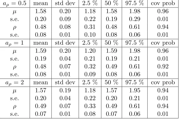
distri-butions with parameters set at µ = π/2 = 1.5708 and ρ = 0.5. In order to study the

sensitivity of priors, we fit each of the three distributions with priors given in equation

(2.2) with aρ = 0.5,1 and 2. We compute the posterior mean, standard deviation, 2.5

percentile, median and 97.5 percentile forµ and ρ for each simulation. The percentiles are

computed with 0 radians as the reference point on the circle. Usually, the reference point

on the circle is chosen diametrically opposite the sample mean, or where the samples are

sparsely distributed. Note that, changing the reference point does not affect the circular

mean. Bayesian highest posterior density (HPD) can be used instead of percentiles. HPD

is unaffected by the change in the reference point. This is described in more detail in

Section 2.7.1. The simulation standard errors for each of these summary values are also

computed. We also compute the nominal coverage probability for the 95% posterior interval

given by the 2.5 and 97.5 percentile of the posterior distribution. In each simulation, we

choose the burn-in period to be 2000 samples (i.e. throw away first 2000 samples from the

MCMC chain) and then keep 5000 samples after burn-in, to obtain posterior summary

val-ues. The sample size was decided after some preliminary studies using Geweke diagnostics,

(34)

Table 2.1: Fitting WN to WN distribution using different priors

aρ= 0.5 mean std dev 2.5 % 50 % 97.5 % cov prob

µ 1.58 0.20 1.18 1.58 1.98 0.96

s.e. 0.20 0.09 0.22 0.19 0.29 0.01

ρ 0.48 0.08 0.31 0.48 0.61 0.94

s.e. 0.08 0.01 0.10 0.08 0.06 0.01

aρ = 1 mean std dev 2.5 % 50 % 97.5 % cov prob

µ 1.59 0.20 1.20 1.59 1.98 0.96

s.e. 0.19 0.04 0.21 0.19 0.21 0.01

ρ 0.48 0.07 0.32 0.49 0.61 0.92

s.e. 0.08 0.01 0.09 0.08 0.06 0.01

µ 1.57 0.19 1.18 1.57 1.95 0.94

s.e. 0.20 0.04 0.22 0.20 0.21 0.01

ρ 0.49 0.07 0.33 0.49 0.61 0.94

s.e. 0.07 0.01 0.08 0.07 0.06 0.01

trace plots. This was done using the CODA program. Tables 2.1 through 2.7 contain all

summary values based on these final 5000 samples. We repeat the entire procedure 500

times to see the frequentist performance of the proposed Bayes method. In SAS, on a sparc

20 machine, on an average it took about 50 minutes to perform the entire simulation for a

given wrapped distribution.

Bayesian highest posterior density (HPD) can also be used instead of percentiles.

For example, in Figure 2.7, we plot the posterior density ofµwhile fitting WC to Ant data.

Since the posterior density has most its mass close to 3.24 radians (185◦), we computed the

percentiles with 0 radians as the reference point. The percentiles will change if we change

the reference point, but the change will be minimal for the Jander’s ant data set, if the

reference point is away from 3.24 radians. However, HPD is not affected by the change in

(35)

Table 2.2: Fitting WC to WC distribution using different priors

µ 1.57 0.17 1.23 1.57 1.92 0.95

s.e. 0.18 0.14 0.20 0.17 0.34 0.01

ρ 0.49 0.07 0.34 0.49 0.61 0.90

s.e. 0.09 0.02 0.10 0.09 0.08 0.01

µ 1.56 0.17 1.23 1.56 1.90 0.93

s.e. 0.17 0.05 0.20 0.17 0.19 0.01

ρ 0.48 0.07 0.33 0.49 0.61 0.94

s.e. 0.07 0.01 0.09 0.07 0.06 0.01

µ 1.57 0.17 1.25 1.57 1.91 0.95

s.e. 0.17 0.13 0.20 0.16 0.34 0.01

ρ 0.49 0.07 0.35 0.49 0.62 0.92

s.e. 0.08 0.01 0.09 0.08 0.07 0.01

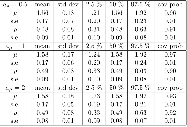
Table 2.3: Fitting WDE to WDE distribution using different priors

µ 1.56 0.18 1.21 1.56 1.92 0.96

s.e. 0.17 0.07 0.20 0.17 0.23 0.01

ρ 0.48 0.08 0.31 0.48 0.63 0.91

s.e. 0.09 0.01 0.10 0.09 0.08 0.01

µ 1.58 0.17 1.24 1.58 1.92 0.97

s.e. 0.17 0.06 0.20 0.17 0.24 0.01

ρ 0.49 0.08 0.33 0.49 0.63 0.90

s.e. 0.09 0.01 0.10 0.09 0.08 0.01

µ 1.58 0.18 1.23 1.58 1.92 0.93

s.e. 0.17 0.05 0.19 0.17 0.21 0.01

ρ 0.49 0.08 0.33 0.49 0.63 0.92

(36)

From Table 2.1, Table 2.2 and Table 2.3, we see that the proposed method performs

very well in terms of maintaining the nominal coverage probability when the underlying

distribution is true. In addition, the posterior mean and median can serve as good point

estimates of the parameters. Although we do not see that the posterior distribution is

sensitive to the choice of the hyper parameteraρ, in general, we would recommendaρ= 0.5

for all the wrapped distributions. Therefore, we use this value for aρ for our application

and other simulations.

In order to study the sensitivity of the sampling distribution, we generated data

from Normal, Cauchy and Double Exponential distributions on the real line and wrapped

them onto the circle (0,2π). For our simulations, we fixedµ=π/2 andρ= 0.5. We

gener-ated n= 50 observations from the W N(π/2,0.5), W C(π/2,0.5) and W DE(π/2,0.5). We

then fitted Wrapped Normal, Wrapped Cauchy and Wrapped Double Exponential

distribu-tions to each of the three datasets. We repeated the method 500 times to see the frequentist

performance of the Bayes method for erroneous models. For model fitting we usedaρ= 0.5

for all priors. In our study (as shown previously in Table 2.1, Table 2.2 and Table 2.3) we

did not find the posterior summary to be very sensitive to the choice of aρ. Therefore, we

did not report the posterior summary values for other choices of aρ. As before, we report

the posterior mean, standard deviation, and two equal tail percentiles along with the Monte

Carlo standard error. Table 2.4, Table 2.5 and Table 2.6 contain the summary statistics.

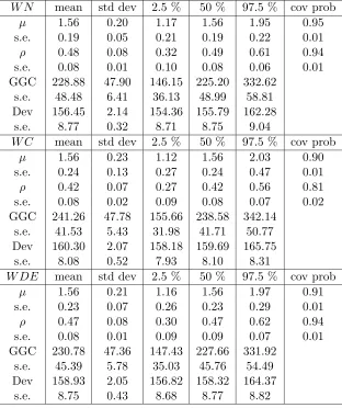
Comparing the results in Table 2.4, Table 2.5 and Table 2.6, we see that the

model selection criteria GGC and deviance work well and select the right distribution. A

(37)

Table 2.4: Fitting WN, WC and WDE to WN distribution withρ∼Beta(0.5,0.5)

W N mean std dev 2.5 % 50 % 97.5 % cov prob

µ 1.56 0.20 1.17 1.56 1.95 0.95

s.e. 0.19 0.05 0.21 0.19 0.22 0.01

ρ 0.48 0.08 0.32 0.49 0.61 0.94

s.e. 0.08 0.01 0.10 0.08 0.06 0.01

GGC 228.88 47.90 146.15 225.20 332.62

s.e. 48.48 6.41 36.13 48.99 58.81

Dev 156.45 2.14 154.36 155.79 162.28

s.e. 8.77 0.32 8.71 8.75 9.04

W C mean std dev 2.5 % 50 % 97.5 % cov prob

µ 1.56 0.23 1.12 1.56 2.03 0.90

s.e. 0.24 0.13 0.27 0.24 0.47 0.01

ρ 0.42 0.07 0.27 0.42 0.56 0.81

s.e. 0.08 0.02 0.09 0.08 0.07 0.02

GGC 241.26 47.78 155.66 238.58 342.14

s.e. 41.53 5.43 31.98 41.71 50.77

Dev 160.30 2.07 158.18 159.69 165.75

s.e. 8.08 0.52 7.93 8.10 8.31

W DE mean std dev 2.5 % 50 % 97.5 % cov prob

µ 1.56 0.21 1.16 1.56 1.97 0.91

s.e. 0.23 0.07 0.26 0.23 0.29 0.01

ρ 0.47 0.08 0.30 0.47 0.62 0.94

s.e. 0.08 0.01 0.09 0.09 0.07 0.01

GGC 230.78 47.36 147.43 227.66 331.92

s.e. 45.39 5.78 35.03 45.76 54.49

Dev 158.93 2.05 156.82 158.32 164.37

(38)

Table 2.5: Fitting WN, WC and WDE to WC distribution with ρ∼Beta(0.5,0.5)

µ 1.57 0.23 1.11 1.56 2.04 0.94

s.e. 0.22 0.10 0.25 0.22 0.36 0.01

ρ 0.45 0.08 0.29 0.46 0.59 0.87

s.e. 0.09 0.01 0.10 0.09 0.07 0.02

GGC 232.80 48.21 148.73 229.32 336.40

s.e. 47.06 5.97 35.22 47.64 56.38

Dev 158.93 2.10 156.84 158.29 164.62

s.e. 9.51 0.32 9.46 9.51 9.65

µ 1.57 0.17 1.23 1.57 1.92 0.95

s.e. 0.17 0.11 0.21 0.16 0.34 0.01

ρ 0.48 0.07 0.33 0.49 0.62 0.89

s.e. 0.09 0.02 0.10 0.09 0.07 0.01

GGC 222.66 43.76 144.79 220.00 315.54

s.e. 40.01 5.06 30.97 40.15 48.86

Dev 154.76 2.07 152.66 154.14 160.27

s.e. 10.71 0.44 10.60 10.72 10.91

µ 1.57 0.18 1.23 1.57 1.92 0.95

s.e. 0.17 0.11 0.20 0.16 0.34 0.01

ρ 0.49 0.08 0.33 0.50 0.64 0.92

s.e. 0.09 0.01 0.10 0.09 0.08 0.01

GGC 221.19 44.46 142.90 218.25 316.11

s.e. 42.38 4.95 32.96 42.76 50.35

Dev 154.95 2.05 152.87 154.34 160.46

(39)

Table 2.6: Fitting WN, WC and WDE to WDE distribution withρ∼Beta(0.5,0.5)

µ 1.58 0.22 1.14 1.58 2.02 0.96

s.e. 0.21 0.09 0.24 0.21 0.31 0.01

ρ 0.46 0.08 0.29 0.46 0.59 0.89

s.e. 0.09 0.01 0.10 0.09 0.07 0.01

GGC 229.32 47.88 146.09 225.76 332.56

s.e. 45.60 6.24 33.76 46.08 55.58

Dev 158.08 2.13 155.99 157.43 163.88

s.e. 9.45 0.34 9.40 9.43 9.70

µ 1.56 0.18 1.22 1.56 1.92 0.96

s.e. 0.17 0.05 0.21 0.17 0.19 0.01

ρ 0.47 0.07 0.32 0.47 0.60 0.92

s.e. 0.08 0.01 0.09 0.08 0.07 0.01

GGC 225.45 44.73 145.81 222.74 320.27

s.e. 37.60 5.07 28.91 37.68 46.19

Dev 156.09 2.09 153.97 155.45 161.63

s.e. 9.32 0.44 9.25 9.30 9.55

µ 1.57 0.17 1.22 1.57 1.91 0.96

s.e. 0.16 0.05 0.20 0.17 0.19 0.01

ρ 0.49 0.08 0.32 0.49 0.64 0.92

s.e. 0.08 0.01 0.10 0.08 0.07 0.01

GGC 221.53 44.91 142.45 218.56 317.35

s.e. 40.95 5.16 31.56 41.31 49.06

Dev 155.61 2.09 153.50 154.98 161.21

(40)

WDE distributions, the model generated from the true distribution has the lowest GGC

and Dev value. Also, both µand ρ have been well estimated, as we have fitted the correct

distribution.

From Table 2.4, Table 2.5 and Table 2.6, we see that in general, the location

parameter is estimated well, even when the models are erroneous. For WN model, coverage

probability of ρ is less than the nominal level. This indicates that WN is not robust in

estimating the mean resultant length when the distribution is not specified correctly. In the

case of fitting WC model to WN data, we see that the mean resultant is not well estimated.

However, WC model performs considerably better while fitting WDE data. This is expected

as WC is closer to WDE than WN. Finally, we see that for WDE model, the parametersµ

and ρ have been well estimated, even when the distribution is incorrect. Therefore, WDE

model is robust in estimatingµ andρ.

We generate data from Von Mises (VM) distribution on the circle(0,2π). To

gen-erate the data from Von Mises distribution, we use the algorithm given by Best and Fisher

(1978). As before we set the µ = π/2 and ρ = 0.5. We fit Wrapped Normal, Wrapped

Cauchy and Wrapped Double Exponential distributions to Von Mises data and repeat the

procedure 500 times to study frequentist performance.

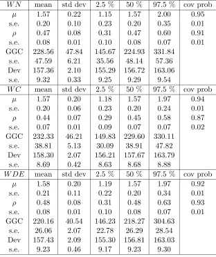
In Table 2.7, we see that WN is robust in estimating µ and ρ when they come

from a Von Mises distribution. This is expected as WN closely approximates the Von Mises

distribution. WC model does not perform well in estimating the mean resultant length. The

lower than nominal coverage probability ofρindicates that WC is not robust in estimating

(41)

Table 2.7: Fitting WN, WC and WDE to VM data with ρ∼Beta(0.5,0.5)

µ 1.57 0.22 1.15 1.57 2.00 0.95

s.e. 0.20 0.10 0.23 0.20 0.35 0.01

ρ 0.47 0.08 0.31 0.47 0.60 0.91

s.e. 0.08 0.01 0.10 0.08 0.07 0.01

GGC 228.56 47.84 145.67 224.93 331.84

s.e. 47.59 6.21 35.56 48.14 57.36

Dev 157.36 2.10 155.29 156.72 163.06

s.e. 9.32 0.33 9.25 9.29 9.54

µ 1.57 0.20 1.18 1.57 1.97 0.94

s.e. 0.20 0.06 0.23 0.20 0.24 0.01

ρ 0.44 0.07 0.29 0.45 0.58 0.87

s.e. 0.07 0.01 0.09 0.07 0.07 0.02

GGC 232.33 46.21 149.83 229.60 330.11

s.e. 38.81 5.13 30.09 38.91 47.82

Dev 158.30 2.07 156.21 157.67 163.79

s.e. 8.69 0.42 8.63 8.68 8.88

µ 1.58 0.20 1.19 1.57 1.97 0.92

s.e. 0.21 0.11 0.22 0.20 0.34 0.01

ρ 0.48 0.08 0.31 0.48 0.63 0.93

s.e. 0.08 0.01 0.10 0.08 0.07 0.01

GGC 220.16 40.54 146.23 218.27 304.63

s.e. 26.06 2.07 22.78 26.29 28.54

Dev 157.43 2.09 155.30 156.81 163.03

Bayesian Analysis of Circular Data Using Wrapped Distributions

Contents

List of Figures

List of Tables

Chapter 1

Introduction to Circular Data

1.1

Some real life applications of circular data

1.2

Statistical Approaches to model circular data

Chapter 2

Parameter Estimation for Wrapped

Distributions

2.1

Previous Work

2.2

The Data Augmentation Approach

2.3

Model selection

2.4

Simulation studies