ABSTRACT
PANSOMBUT, TATDOW. Advanced Learning Techniques for Improved Inference of Bayesian Belief Networks from Uncertain and High-dimensional Data. (Under the direction of Prof. Nagiza F. Samatova and Prof. Dennis R. Bahler.)
A Bayesian Belief Network (BBN) is a powerful probabilistic learning model, it has been
used successfully in many problem domains, such as medical diagnostics, computational
biol-ogy, bioinformatics, image processing, and gaming. The success of Bayesian Belief Networks is due to a number of factors. A Bayesian Belief Network is capable of learning under uncertainty
and can handle many types of data. It is also robust to model overfitting. However, the most
powerful strength of a Bayesian Belief Network is, arguably, its ability to incorporate prior knowledge into the learning process; this characteristic is very unique to a Bayesian learning
model.
To learn a Bayesian Belief Network from data, there are two aspects of learning: (1) learning
the network structure and (2) learning the conditional probabilities of variables in the network.
Learning the conditional probabilities is relatively simple if we know the network structure; however, structure learning is an NP-hard problem. The reason is that the number of network
structures grows super-exponentially in terms of the number of variables (features) in the
net-work. Unfortunately, in some real world problem domains, it is not uncommon for a problem to have a large number of variables. Some of the reasons that contribute to a large number of
variables in a problem are that (1) the problem is underdetermined, (2) the problem contains many irrelevant features, and (3) the problem contains some redundant features.
In this research, we are interested in enhancing the learning ability of a Bayesian Belief Network by incorporating the knowledge obtained from other learning models. We improve (1)
the BBN’s performance in terms of its prediction accuracy and computational learning time
and (2) the BBN’s ability to learn complex and interesting relationships among its variables. We achieve these milestones through the following three complementary approaches that allow
for uncovering some hidden knowledge about data using various supervised and unsupervised
learning models and for using that knowledge to limit the search space for network structure inference.
Component 1: Using a decision tree supervised learning model, we found an informative way to identify the lesser number of discriminatory features used as input for Bayesian Belief
magni-tude and/or increased robustness and accuracy of a Bayesian Belief Network as a classifier.
Component 2: Generalizing our method in Component 1 to highly underdetermined
prob-lems, we developed a method for constructing an ensemble of smaller-size BBN classifiers. This
reduced the learning time and increased the prediction accuracy of a BBN classifier model for unconstrained problems.
Component 3: For underdetermined problems with complex relationships between the data features and data samples, we designed a methodology for explicitly incorporating the
knowl-edge learned about bicluster relationships into the ensemble of BBN classifiers. We were able
to increase the prediction accuracy of a BBN classifier by learning complex relationships from the data that, otherwise, would not be identified when all examples were considered at once.
© Copyright 2011 by Tatdow Pansombut
Advanced Learning Techniques for Improved Inference of Bayesian Belief Networks from Uncertain and High-dimensional Data
by
Tatdow Pansombut
A dissertation submitted to the Graduate Faculty of North Carolina State University
in partial fulfillment of the requirements for the Degree of
Doctor of Philosophy
Computer Science
Raleigh, North Carolina
2011
APPROVED BY:
Prof. Anatoli Melechko Prof. James Lester
Prof. Nagiza F. Samatova Co-chair of Advisory Committee
BIOGRAPHY
Tatdow Pansombut received her Bachelor of Science in Computer Science from Washington
University in St. Louis in Summer 2001. She continued her study at Washington University in St. Louis and earned her Master of Science in Computer Science in Spring 2003. During
her undergraduate and graduate studies at Washington University in St. Louis, she served as a
Teaching Assistant in Advance Algorithms and Formal Foundation of Computer Science. She was admitted to North Carolina State University in Fall 2003 and passed the Written Qualifier
in Spring 2005 under the guidance of Dr. Dennis R. Bahler. She served as a Teaching Assistant
for Data Structures for Computer Scientists, Software Engineering, Design and Analysis of Al-gorithms, and Computational Methods for Molecular Biology from Fall 2005 to Spring 2007.
She was nominated by Dr. Rada Y. Chirkova for an Outstanding Teaching Assistant award
in Fall 2006. She worked as an intern for Sony Ericssion Mobile Communication in Fall 2007. She started working as a Research Assistant for Dr. Nagiza F. Samatova in Fall 2009. Under
Dr. Samatova’s and Dr. Bahler’s guidance, she was able to completed the Oral Examination
in Spring 2010.
Appointments and Tenure
(2009-2011) Research Assistant at North Carolina State University under Dr. Nagiza F. Samatova
(2005-2007) Teaching Asistant at North Carolina State University
(2007, Fall) Member of IP Multimedia Subsystems (IMS) Development Team at Sony Ericsson Mobile Communication
(2000-2002) Teaching Asistant at Washington University
(2001, Fall) Research Assistant at Washington University in St. Louis under Dr. Jeremy Buhler
Supporting Publications
T. Pansombut, W. Hendrix, Z. J. Gao, B. E. Harrison, and N. F. Samatova. “Biclustering-driven ensemble of Bayesian Belief Network classifiers for underdetermined problems,”
The Twenty-Second International Joint Conference on Artificial Intelligence (IJCAI), Barcelona, Spain, July 16-22, 2011.
ACKNOWLEDGEMENTS
I would like to thank both of my advisors, Prof. Nagiza Samatova and Prof. Dennis Bahler for
their guidance, support, and patience. I would not be able to complete this work without their help. I would also like to thank my PhD committee members, Prof. James Lester and Prof.
Anatoli Melechko, for their helpful suggestions and questions.
I would like to thank my fellow graduated students whom I have a great opportunity to work with, William Hendrix, Zhengzhang Chen, Huseyin Sencan, Pu Yang, Doel Gonzalez, and Brent
Harrison.
I would like to thank all of my friends, especially David Brossoie and Joey Kam, who have been great support for me. Last, I would like to thank my family, especially my mother, my aunt,
TABLE OF CONTENTS
List of Tables . . . vii
List of Figures . . . .viii
Chapter 1 Introduction . . . 1
1.1 Feature Selection using Decision Tree . . . 2
1.2 Iterative Decision Tree Feature Knock-Out for Ensembles of Bayesian Belief Net-work Classifiers . . . 4
1.3 Biclustering-Driven Ensemble of Bayesian Belief Network Classifiers for Under-determined Problems . . . 5
Chapter 2 Decision Tree based Feature Selection . . . 6
2.1 Feature Selection . . . 6
2.1.1 Filter Feature Selection . . . 8
2.1.2 Wrapper Feature Selection . . . 9
2.1.3 Hybrid Feature Selection . . . 9
2.1.4 Embedded Feature Selection . . . 10
2.2 Methodology . . . 10
2.3 Results . . . 14
2.3.1 Data . . . 14
2.3.2 Evaluation Methodology . . . 14
2.3.3 Comparison of Time Efficiency between C4.5 Decision Tree Classifier and Bayesian Classifiers without Feature Selection . . . 15
2.3.4 Comparison of Time Efficiency between Bayesian Classifiers with and without Feature Selection . . . 16
2.3.5 Comparison of Accuracy between Bayesian Classifiers with and without Feature Selection . . . 16
2.3.6 The Number of Features Reduced by C4.5 Decision Tree . . . 19
2.4 Discussion and Related Work . . . 19
2.5 Conclusion . . . 22
Chapter 3 Iterative Decision Tree Feature Knock-Out for Ensembles of Bayesian Belief Network Classifiers . . . 24
3.1 Problem and Proposed Solution . . . 24
3.2 Ensemble Methods . . . 26
3.2.1 Ensemble Methods for “Weak” or “Unstable” Classifiers . . . 27
3.2.2 Ensemble Method for Reducing the Expected Error . . . 28
3.2.3 Ensemble Methods for Problematic Data . . . 29
3.2.4 Weighting Schemes for Improving the Prediction Accuracy of Ensemble Methods . . . 29
3.3 Methodology . . . 30
3.3.2 Iterative Decision Tree Feature Knock-Out Method . . . 32
3.3.3 Ensemble of BBN Classifiers . . . 32
3.3.4 Model Selection . . . 33
3.3.5 Creating and Weighting the Ensemble . . . 33
3.3.6 Algorithm . . . 34
3.4 Results . . . 35
3.4.1 Data . . . 35
3.4.2 Experimental Methodology . . . 35
3.4.3 Prediction Accuracy . . . 36
3.4.4 Learning Time . . . 37
3.5 Related Work . . . 37
3.6 Conclusion . . . 37
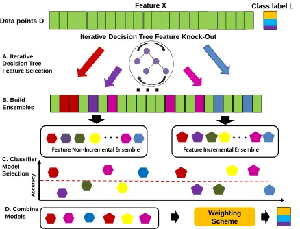
Chapter 4 Biclustering-Driven Ensemble of Bayesian Belief Network Classi-fiers for Underdetermined Problems . . . 39
4.1 Problem and Proposed Solution . . . 39
4.2 Method . . . 41
4.2.1 Overview . . . 41
4.2.2 Biclustering Data . . . 42
4.2.3 Calculating Bicluster Enrichment . . . 42
4.2.4 Combining Biclusters . . . 43
4.2.5 Creating and Weighting the Ensemble . . . 44
4.3 Results and Discussion . . . 44
4.3.1 Data . . . 44
4.3.2 Overall BENCH Performance . . . 44
4.3.3 Different Weighting Schemes . . . 46
4.3.4 Parameters for Random Forests . . . 46
4.3.5 FI and FE Classifiers . . . 46
4.3.6 Learning Time . . . 47
4.4 Related Work: BBN ensemble classification . . . 49
4.5 Generalization of BENCH to other Classifiers . . . 51
4.6 Conclusion . . . 51
Chapter 5 Conclusion and Future Work . . . 52
5.1 Future Work for BBN-ITDT Algorithm . . . 52
5.2 Future Work for BENCH . . . 53
5.3 Future Work for BBN-ITDT Algorithm and BENCH . . . 53
References. . . 55
Appendices . . . 61
Appendix A . . . 62
LIST OF TABLES
Table 2.1 Datasets Information . . . 13
Table 2.2 BBN Learning Algorithms Information . . . 13
Table 2.3 Learning Time of BBN without Feature Selection (seconds) . . . 15
Table 2.4 Learning Time of BBN using Feature Selection (seconds) . . . 17
Table 2.5 BBN Classification Accuracy with and without Feature Selection (FS) . . 18
Table 2.6 Number of Features Before and After Decision Tree Feature Selection . . 19
Table 2.7 Features and Training Sets Comparisons of Filter Based Feature Selection Algorithms and C4.5 Decision Tree . . . 19
Table 2.8 Accuracy Comparison of Filter Based Feature Selection Algorithms and C4.5 Decision Tree . . . 20
Table 3.1 Compare Prediction Accuracy for Underdetermined Problems . . . 25
Table 3.2 Description of Notations Used in Chapter 3. . . 30
Table 3.3 Dataset Information . . . 35
Table 3.4 Compare Prediction Accuracy . . . 36
Table 4.1 Description of Notation Used in Chapter 4 . . . 40
Table 4.2 Comparison of prediction accuracy for different weighting schemes on Leukemia, Lymphoma Survivor, and Colon Cancer datasets . . . 46
LIST OF FIGURES
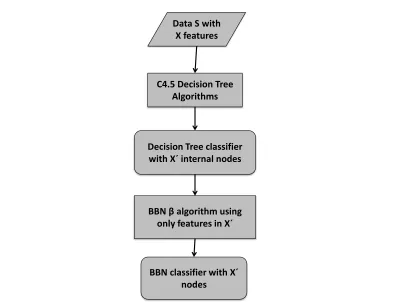
Figure 2.1 Flow Chart of Decision Tree Feature Selection for BBN Classifier Algo-rithm (BBN-DT) . . . 12
Figure 3.1 Flow Chart of Iterative Decision Tree Feature Knock-Out for Ensembles of BBN Classifiers Algorithm (BBN-ITDT) . . . 31
Figure 4.1 Flow Chart of Biclustering-driven ENsemble of BBN Classifiers Algo-rithm(BENCH) . . . 41 Figure 4.2 Comparison of prediction accuracy of BENCH to single and ensemble
classifiers on the Leukemia dataset . . . 45 Figure 4.3 Compare Prediction Accuracy of Different Parameters (no. of Classifiers
and no. of Features) for Random Forest on Leukemia Dataset . . . 47 Figure 4.4 Comparison of prediction accuracy between FI and FE classifiers using
confidence weighting on Leukaemia, Lymphoma Survivor, and Colon Can-cer datasets . . . 48 Figure 4.5 Compare Learning Time of Single and Ensemble BBN Classifiers on Leukemia
Chapter 1
Introduction
Learning under uncertainty is an important field in machine learning because the aim in machine learning is for an artificially intelligent (AI) agent to act rationally by learning to adapt to new
circumstances and extrapolate patterns [1]. If all the relevant facts are known, then an agent
can learn to derive a logical plan to achieve its goal. However, in real world applications, the agent rarely has access to all the facts. Without that information, how can the agent learn to
act rationally?
Many learning models have been developed to address the problem of learning under uncer-tainty. Some examples of those models are the Dempster-Shafer theory, Rule-based approach,
and Fuzzy logic [1]. However, one of the most widely-used and successful models in learning
un-der uncertainty is a graphical probabilistic model known as a Bayesian Belief Network (BBN). The reason for its success may be due to some of the characteristics of the Bayesian Belief
Network learning model [2] [3], including but not limited to the following:
1. A Bayesian Belief Network is able to learn multiple hypothesis models at the same time
by increasing its belief in each model without completely eliminating a hypothesis model that is inconsistent with some examples.
2. A Bayesian Belief Network can make probabilistic predictions.
3. A Bayesian Belief Network, although often computationally intractable, is well-studied and many learning techniques have been developed to learn this model.
4. A Bayesian Belief Network provides an approach to combine prior knowledge with
ob-servable data.
5. A Bayesian Belief Network is able to handle incomplete data.
7. A Bayesian Network is robust to model overfitting.
Because of the above characteristics, a Bayesian Belief Network is a powerful tool in learning
under uncertainty in many areas. The two main applications of a Bayesian Belief Network in machine learning are:
1. Using a Bayesian Belief Network for supervised learning classification.
2. Discovering and representing dependency relationships among variables (attributes or features) in the problem domain.
In this research, we are interested in improving both applications of a Bayesian Belief
Net-work. Particularly, we aim to improve the performance in terms of the required computational
time and accuracy of a Bayesian classifier, and to advance its ability to learn complex relation-ships from real world data. We plan to achieve our goal by incorporating someprior knowledge from other learning models.
To improve the accuracy of and to reduce the amount of learning time required by a Bayesian classifier, we use a supervised learning method, known as a decision tree classifier, to select the
most “relevant” features for a Bayesian Belief Network learner. See Chapter 2 for more detail.
To improve the accuracy and reduce the amount of time when learning underdetermined problems (problems that contain a larger features than data points), we use the idea of ensemble
methods to build an ensemble of classifiers. This method will construct multiple Bayesian-based
classifiers from various subsets of features selected by the Iterative Decision Tree Feature Knock-Out algorithm. See Chapter 3 for more detail.
To further improve the accuracy of Bayesian Belief Network classifiers and to enable the
learning of complex relationships among the variables and the data samples in the application domain, we plan to combine an unsupervised learning method, known as a biclustering method
with a supervised learning model of a Bayesian Belief Network. Specifically, we utilize the
strength of a biclustering method to uncover interesting patterns within subsets of data points and subsets of features and use these patterns (along with the class label) to build an ensemble
of Bayesian Belief Network classifiers. See Chapter 4 for more detail.
Next, we would like to give a brief summary of the problems, proposed approaches, and research challenges to our research questions.
1.1
Feature Selection using Decision Tree
Problem:
A Bayesian Belief Network is a great choice for a classifier when learning under uncertainty,
or continuous). Moreover, performing an inference in a Bayesian Belief Network is fast and
the conditional probabilities can easily be updated when new evidence is presented after the structure of the network is known.
However, finding a structure of the network is a time consuming task; this problem is an
NP-hard problem [4]. Many heuristic algorithms, such as Hill Climbing, Simulate Annealing, TAN, and Conditional Independence Test [5] have been developed to learn the structure of
the network in a more efficient way. The reason is that the search space for putative network
structures grows super-exponentially in terms of the number of variables in the domain [6]. One solution is to reduce the number of variables before building the network structure by
identifying the discriminating variables (features) for a particular dataset.
Approach:
In this research, we propose to identify the discriminating features by using a decision tree
classifier. A Bayesian Belief Network is typically used to learn the relationships of the variables (features) in the problem domain when we believe many of those variables to be independent
of each other. In this case, we expect to have a relatively few edges in the network when
Bayesian Belief Network structure learner attempts to determine the relationship between any two variables in the domain from a given dataset, some of those variables may be strongly
correlated while others are not.
This knowledge raises the question: is it possible to ignore the weakly co-related
relation-ships while building a Bayesian classifier without sacrificing performance? One approach to
reducing the weakly co-related relationships in the network is to identify a subset of variables (features) that are not strongly co-related to other variables. If we can find such a subset,
then we can remove these variables from the dataset prior to the construction of the network
structure. If we can retain or even improve the performance of the Bayesian classifier, then we can conclude that the remaining variables in the network are the features that discriminate the
data points.
Our method proposes to use a decision tree classifier to identify the discriminating features in the problem domain. In a decision tree classifier, the features that are better at
distinguish-ing the data points are closer to the root of the tree. Because a decision tree classifier has
a tendency to overfit the training set, a technique known as pruning reduces the height of a decision tree by removing some branches of the tree, and replacing them with leaves (in effect
removing some features in the tree) in order to overcome the overfitting problem. To develop
Research Questions:
1. How does the performance of the decision tree classifier (used for feature selection) affect the performance of the Bayesian classifier?
2. What kinds of problem domains are more likely to succeed with this approach?
3. How does the choice of Bayesian classifier learning algorithms affect the performance of
the classifier? What characteristics of Bayesian learning algorithms are more suitable with this approach and why?
1.2
Iterative Decision Tree Feature Knock-Out for Ensembles
of Bayesian Belief Network Classifiers
Problem:In some real world problem domains, learning to construct an accurate classifier may be a very difficult task due to the nature of the data. The reason is that the datasets derived from
real world problem domains like biology or climatology may present the learner with
underde-termined problems (problems that contain more features than data points). Underdeunderde-termined problems are hard to learn because (1) the limited number of data points is not sufficient to
provide the learner with enough information to build an accurate classifier and (2) the large
number of features requires considerable amount of learning time (especially for BBN classifiers).
Approach:
One possible solution is to consider an ensemble method. We propose to build an ensemble of BBN classfiers with sets of features that are selected by a decision tree algorithm. In order to
produce multiple sets of discriminating features, we will apply the decision tree algorithm to a
dataset in an iterative manner. To explore this approach, we addressed the following questions (see Chapter 3 for more details).
Research Questions:
1. How should we use the sets of discriminating features (selected by decision tree classifier)
to build an ensemble of BBN classifiers?
2. What should the size of an ensemble be in order to build an accurate classifier?
3. It is possible to select too many features that may lead to overfitting?
1.3
Biclustering-Driven Ensemble of Bayesian Belief Network
Classifiers for Underdetermined Problems
Problem:
In addition to the issues that arise from problematic data, there are problems due to the
complexity of the relationships between the features in data that we aim to learn. In
tra-ditional Bayesian network structure learning, an algorithm typically attempts to identify the dependency relationships among features that are present across all data points. However, in
some problem domains (like Inference of Transcriptional Gene Networks), we may be interested in the kind of relationships that exist when considering only subsets of the data points with the
corresponding subsets of features. These types of relationships are hard to discover, because
the signal is not strong enough when all the data points and all the features get considered at once. How can a learner discover this type of relationship? Would it be possible to use our
knowledge about this type of relationship to improve the performance of a BBN classifier?
Approach:
In this research, we incorporate knowledge obtained from a biclustering method to build an
ensemble of BBN classifiers. We use biclustering as a tool to uncover the kind of relationships that only exist between subsets of features and/or subset of data points. We use the knowledge
about these relationships to guide us on how to build an ensemble of classifiers. To explore this
approach, we need to address the following research questions (see Chapter 4 and our accepted manuscript [8] for more details).
Research Questions:
1. How should we use the result obtained from biclustering method to build an ensemble of
BBN classifiers?
2. How can we incorporate the result from an unsupervised learning model (biclustering) to the learning of a supervised learning model (BBN)?
3. Can we improve the performance of a BBN classifier if we have the knowledge about the complex relationships that exist between its subsets of variables and subsets of data
Chapter 2
Decision Tree based Feature
Selection
In this chapter, we improve the performance of a Bayesian classifier by using a decision tree
classifier as a feature selection technique to identify a subset of discriminating features. Before
we describe our method and result, we would like to discuss the concept of feature selection and how feature selection techniques have been used in relation to a Bayesian classifier. In addition,
we will give a brief introduction to a decision tree classifier.
2.1
Feature Selection
Feature selection is an important field in machine learning because of the rise in mass quantity of
data from corporate and scientific records and in low quality data from the World Wide Web [9]. Feature selection techniques are developed in the fields of pattern recognition, machine learning,
data mining, and bioinformatics and successfully applied to the fields of image retrieval, genomic
analysis, text categorization, and intrusion detection [10] because of their many advantages [11], including but not limited to the following.
1. Feature selection helps to avoid overfitting and improve the performance of the learning
model.
2. Feature selection reduces the complexity of the learning model.
3. Feature selection helps to gain a deeper understanding of the underlying process that
generates the data.
4. Feature selection preserves the semantics of the variables (features) which allows domain
Feature selection or feature subset selection is a data preprocessing technique [10] that
reduces the number of features in the problem domain by removing irrelevant features and redundant features. Irrelevant features are features that contain no useful information for the target concept and redundant features are features that contain much or all information in-cluded in another feature or subset of other features [3]. After removingirrelevant features, and redundant features, what remains is a set ofrelevant features.
In this chapter, we are primarily concerned with feature selection for the purpose of classi-fication. In this context, arelevant feature is defined in terms of its relation to a target concept as follows.
Let D be a set of feature set values over a set of featuresX, letY be a set of class labels,
and let L be the associated class label function such thatL:D→Y. Let S ={(di, li)|di ∈D and li ∈L} be a training set of data points (or sample set). A target concept T is a function that maps a feature set value to a class label (T : D → Y). A data point in S is generated from an instance space with a joint probability distribution D,L. A target conceptT is what
we want to learn. A feature x∈X is relevant to a target concept T, if there exists a pair of examples di and dj in an instance space such that di and dj only differ in
their assignments in x and T(di)6=T(dj) [9].
For a classification problem, we aim to improve the performance of a classifier by using
feature selection to identify a set ofrelevant features. We expect this approach to increase the accuracy of the classifier by avoiding overfitting and by making the classifier more robust to
noise in the data, to reduce the computational learning time by limiting the search space, to
decrease the classification time by simplifying the complexity of the model, and to facilitate the interpretability of the derived relationships between the features.
A typical feature subset selection process usually contains four components [10].
1. Subset generation is the process that defines the starting point of the search and gener-ates candidate subsets to be evaluated by the next subset evaluation. Some techniques
for generating candidate subsets are sequential search methods like sequential forward
se-lection and sequential backward elimination or random search methods like random start and simulated annealing.
2. Subset evaluation is the process by which each candidate subset is evaluated by evaluation criteria. The evaluation criteria may be independent or dependent from the inductive
3. Stopping criterion determines when the feature selection process should stop. Some
ex-amples for stopping criteria are when the search is complete, when a priori given bound is reached, when subset generation cannot produce better candidates, or when the inductive
algorithm attains certain accuracy.
4. Result validation is the process in which we measure the quality of the resulting feature
subset either by comparing the resulting feature subset to the known relevant features (for a simulated dataset) or by comparing the accuracy of the classifier learned by using
the resulting subset with the one learned by using the full feature set (for a real world
dataset).
Many feature selection techniques have been developed for machine learning. There are
four main classes of feature selection techniques in machine learning literature, each depending on how the techniques combine the feature selection process with the learning process of the
inductive algorithms [11]. In the next four subsections we will discuss the four feature selection classes (Filter, Wrapper, Hybrid, and Embedded) in terms of their characteristics, advantages,
and disadvantages. We will also give some example algorithms of each technique.
2.1.1 Filter Feature Selection
In the filter feature selection approach, the feature selection process is done prior to the con-struction of the classifier. The search space for feature subsets is separated from the search
space for the classifiers. The filter approach looks into the intrinsic properties of the data [11],
and measures the relevant score of an individual feature or a subset of features using some mea-surement related to the target concept [9]. This approach makes the feature selection process
independent of the inductive learning algorithms.
The advantages of this approach are the following: (1) it is fast, (2) it is scalable, (3)
it is independent on the classifiers. However, it has a number of disadvantages including the following: (1) it ignores the feature dependency and (2) it ignores feature and model
depen-dency [11]. In some cases, the performance of the classifier may suffer as the result of ignoring
these dependencies.
2.1.2 Wrapper Feature Selection
In the wrapper feature selection approach, the feature selection process generates various
candi-date feature subsets from the current chosen subset, and these subsets are evaluated by training
and testing sets using a specific classifier. A new feature subset with the best performance is chosen from the candidate subsets, and the process is repeated if the stopping criteria is not
met. With this approach, the search space for the features is wrapped around the search space
for the classifiers.
The advantages of the wrapper approach are the following: (1) it is simple, (2) it allows
the interaction between feature selection and model selection, and (3) it can model feature dependency. The disadvantages of this approach are the following: (1) it has higher risk of
overfitting than the filter method, (2) it is dependent on the choice of a classifier, and (3) it is usually computationally-intensive (although much research has focused on reducing the size of
testing sets to decrease the computational time) [11].
Some examples of the wrapper feature selection are sequential forward selection [16],
se-quential backward elimination [16], plus q take-away r [17], beam search [18], simulated
an-nealing, randomized hill climbing [19], genetic algorithms [20], and OBLIVION (wrapper for nearest-neighbor method) [11].
2.1.3 Hybrid Feature Selection
The hybrid feature selection approach combines the strengths of the filter and wrapper methods.
This technique iterates through the cardinalities of features subsets. It uses the filter method to evaluate the best subset for each given cardinality starting with the subset of size zero. In each
iteration, it finds the best subset of the current cardinality, then searches through all possible
subsets of the next cardinality (incremented by one) by adding the remaining features to find the best subset of the next cardinality using filter method. The best subsets of the current
and next cardinalities are trained and tested using some classifier. If the current cardinality subset performs better than the next one, then the search stops, otherwise, it continues by
incrementing the current cardinality by one [10].
The advantages of the hybrid method are the followings: (1) it is less computationally
intensive than the wrapper method, (2) it allows some interaction between model and feature
An example of this approach is the symmetrical uncertainty genetic algorithm wrapper
[21].
2.1.4 Embedded Feature Selection
In the embedded feature selection approach, the feature selection process is built into the
pro-cess of constructing the classifier. The inductive algorithm incorporates feature selection into
the learning algorithm by combining the search space of feature subsets to the search space of classifiers. The advantages of this approach are that (1) it permits interaction between model
selection and feature selection, (2) it allows the ability to model features and model depen-dency, and (3) it generally has better computational complexity than the wrapper method [11].
However, it has a disadvantage in that the feature selection process is very dependent on the
inductive learning algorithms.
Some example algorithms of this approach are the greedy set-cover algorithm, an algorithm
for learning k-term Disjunctive Normal Form (DNF) formulae [22], the inductive decision tree learning algorithms (ID3 [23], C4.5 [24], and CART [25]), and the separate-and-conquer
meth-ods for learning a decision list [26] [27] [28]. In general, the embedded approach works well
when there is little interaction between features [9].
2.2
Methodology
In this research, we propose a new strategy to use decision tree classification as a filter feature
selection method to improve the performance of Bayesian classifiers. The reason for choosing a filter feature selection approach is the following. Filter feature selection is fast and scalable.
These characteristics are quite opposite to the ones of a Bayesian classifier. Learning a Bayesian classifier is not a simple task, it can be very time and memory consuming, especially, when the
number of features is large, because the number of putative Bayesian network structures forN
features is in the order ofO(2N2) [6]. Our goal is not only to find a good feature subset, which will result in decreasing the classifier learning time, but also to find such a subset fast.
Consider a problem domain containing N features, when N0 is the size of an optimal fea-ture subset. If N is significantly larger than N0 (N N0), then finding a good feature subset using a sequential backward elimination wrapper method would be time consuming, since we
have to start with the full feature set. Even if we use a sequential forward selection wrapper method, we are still faced with the problem of overfiting and dependency on the order that
to modify an existing Bayesian classifier learning algorithm to incorporate a feature selection
task. This approach is not only complicated, but also it is dependent on the choice of the learning algorithm. A hybrid method would have been a better choice; however, it would have
been slower than the filter one. Therefore, a filter feature selection approach seems like a
bet-ter choice for a classifier that is potentially as time consuming to learn as a Bayesian classifier is.
The next question is why do we choose a decision tree classifier as a our feature selection
mechanism? An answer is due to the following interesting observations:
1. Decision tree learners require no prior knowledge about prior probability distribution, while Bayesian learners have the advantage of incorporating prior knowledge.
2. Decision tree learners are often fast and computationally inexpensive, while Bayesian
learners are not.
3. Decision tree learners usually maintain a single hypothesis, while Bayesian learners are
capable of maintain multiple ones.
What we propose is to combine the strengths of the two successful complementary learning tools in an intuitively simple way. It is simple, because we do not need to modify any existing
Bayesian classifier algorithms. A Bayesian learner can take advantage of the prior knowledge (which is a good feature subset) learned by a decision tree learner. Since decision tree learning is fast and computationally inexpensive, it is expected not to significantly increase the amount
of time and resources already required by a Bayesian learner. In addition, we should be able to take advantage of maintaining multiple hypotheses.
Given our justified choice of a feature selection technique (a filter feature selection approach) and a tool (a decision tree classifier), we will next give an overview of our strategy and some
intuition behind it. Please refer to Flow Chart 2.1 and Algorithm 1, the Decision Tree Feature
Selection for BBN Classifier Algorithm (BBN-DT).
The Decision Tree Feature Selection for BBN Classifier Algorithm takes a training set of
data pointsS over the set of variables (features)X and a Bayesian classifier learning algorithm
β as input (for the information about these algorithms, please refer to Appendix A). It first
constructs a decision tree classifier fromS using the full feature set, and output a decision tree
classifier T (Lines 2-4). The algorithm then constructs a Bayesian classifier B from S using only features from the internal nodes of T (Line 6). It returns a BBN classifier B and a set of
C4.5 Decision Tree Algorithms Data S with
X features
Decision Tree classifier with X´ internal nodes
BBN β algorithm using only features in X´
BBN classifier with X´ nodes
Figure 2.1: Flow Chart of Decision Tree Feature Selection for BBN Classifier Algorithm (BBN-DT)
Require: X: a set of features
Require: S: a set of data points overX and the class labels Require: L: a class label function for all data points inS
Require: β: a Bayesian classifier learning algorithm which produces a BBN classifier
Ensure: B: a BBN classifier Ensure: X0: a subset ofX
1: B = NULL
2: Run the decision tree learning algorithm on S
3: Output a decision tree T
4: Let X0 be a set of all features that belong to the internal nodes ofT
5: Let S0 be a set of data points containing all data points inS but only features inX0
6: Run algorithmβ on S0 to produce B = (Bs,Θ)
7: return (B, X0)
Table 2.1: Datasets Information
Dataset Data points Feature Class Missing value Numeric features
Breast 198 34 2 yes yes
Chess 3195 37 2 no no
Credit 690 16 2 yes yes
Mushroom 8124 23 2 yes no
Splice 3189 61 3 no no
Soybean 306 36 19 yes no
Voting 435 17 2 yes no
Table 2.2: BBN Learning Algorithms Information
Algorithm Type Max no. of parents Sensitive to variable ordering
K2 local search 5 yes
HCa local search 5 no
RHC b local search 5 no
LHC c local search 5 no
TSd local search 5 no
SN e local search N/A no
TAN CITg N/A no
CIf CITg N/A no
ICS CITg N/A no
aHill Climber
bRepeated Hill Climber
cLook Ahead in Good Direction (LAGD) Hill Climber dTabu Search
eSimulated Annealing fConditional Independence g conditional independent test
We use a C4.5 decision tree classifier and nine Bayesian classifier learning algorithms(see Table 2.2) on the full feature sets of four datasets (see section 4.3 for more details). Because the
C4.5 decision tree learning algorithm prunes the tree after it is built, we expect to find some
features that are excluded from the decision tree. We run the same Bayesian classifier learning algorithms using only these features included in the pruned decision tree for each dataset. Since
our goal is to improve the performance of Bayesian classifiers, we record the learning times and
2.3
Results
2.3.1 DataWe ran experiments using seven datasets from the UCI Machine Learning Repository [29],
nam-ily, Breast, Chess, Credit, Mushroom, Splice, Soybean and Voting. Table 3.3 provides informa-tion about the number of data points, the number of features, the number of class attributes,
whether the datasets contain any missing attribute values, and whether the datasets contain any numeric (continuous) attribute values. Our main experiments focus on four datasets: Breast,
Credit, Mushroom, and Voting. The experiments involving the Chess, Spice, and Soybean
datasets are for the purpose of comparison to related works. We choose Breast, Credit, Mush-room, and Votintg datasets for their varieties, and because they are often used in Bayesian
Belief Network related-research experiments. It is important to note that the datasets are
pre-processed prior to the learning process by replacing any missing values with the most common one and by discretizing the continuous attributes.
2.3.2 Evaluation Methodology
In order to evaluate our approach, we ran the experiments using the following criteria.
1. We ran the experiments on heterogeneous types of datasets, some of them containing
missing attribute values.
2. We compared the performance of nine Bayesian classifier learning algorithms whenever
applicable.
3. We used a reliable and widely-used machine learning toolkit, WEKA [30].
4. We evaluated the performance using a 5-fold cross validation method.
In addition, our experiments were designed to answer the following questions.
1. How does the particular choice of a learning algorithm affect our approach?
2. What is the percentage of feature reduction required for our method to be effective? Is it
possible and/or desirable to reduce too many features?
3. What is the relation between the number of features being reduced and the performance
increase/decrease?
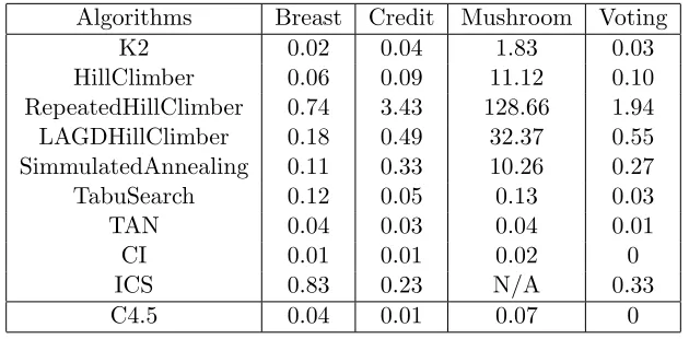
Table 2.3: Learning Time of BBN without Feature Selection (seconds)
Algorithms Breast Credit Mushroom Voting
K2 0.02 0.04 1.83 0.03
HillClimber 0.06 0.09 11.12 0.10
RepeatedHillClimber 0.74 3.43 128.66 1.94 LAGDHillClimber 0.18 0.49 32.37 0.55 SimmulatedAnnealing 0.11 0.33 10.26 0.27
TabuSearch 0.12 0.05 0.13 0.03
TAN 0.04 0.03 0.04 0.01
CI 0.01 0.01 0.02 0
ICS 0.83 0.23 N/A 0.33
C4.5 0.04 0.01 0.07 0
5. What computational benefits can be offered by our approach?
2.3.3 Comparison of Time Efficiency between C4.5 Decision Tree Classifier and Bayesian Classifiers without Feature Selection
From our experiments, we observe that the decision tree classifier is able to reduce the number
of features for four datasets (Breast, Credits, Mushroom, and Voting). From the time efficiency
perspective, the summary of the results for these four datasets displayed in Table 2.3 is the following:
1. For the Breast and Credit datasets, the decision tree classifier outperformed all of the
Bayesian classifiers, except for the CI algorithm.
2. For the Mushroom dataset, the decision tree classifier outperformed all of the Bayesian classifiers, except for ICS algorithm, for which the data is not available.
3. For the Voting dataset, the decision tree classifier outperformed nine of the Bayesian classifiers, except for the CI algorithm, which performed as well as the decision tree
classifier.
It is interesting to note that both CI, ICS, and TAN use conditional independence to
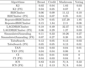
2.3.4 Comparison of Time Efficiency between Bayesian Classifiers with and without Feature Selection
For this experiment, we compared the time required for learning a Bayesian classifier without feature selection with the time required for selecting the features and then learning a Bayesian
classifier on a reduced feature set. Table 2.4 summarizes the results of this comparison.
1. For the Breast dataset, Bayesian classifiers with feature selection perform better than
without feature selection, except for K2 and CI algorithms.
2. For the Credit dataset, Bayesian classifiers with feature selection perform better than
without feature selection, except for the K2, TAN, and CI algorithms.
3. For the Mushroom dataset, Bayesian classifiers with feature selection perform better than without feature selection, except for the CI algorithm.
4. For the Voting dataset, Bayesian classifiers with feature selection outperform or perform
as well as the same algorithm without feature selection, except for K2 algorithm.
From this summary, we can conclude that Bayesian classifiers with feature selection, in most
cases, outperform the ones without feature selection; they often offer an order of magnitude
improvement in time efficiency. There are very few instances when the performance is compa-rable or slightly worsened, but since the overall learning time for such cases is on the order of
the tens or hundredth of a second, such minor degradation is likely due to the overhead time
required to interface between the feature selection algorithm and the classifier. Quantifying this overhead is the subject of our future work.
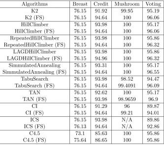
2.3.5 Comparison of Accuracy between Bayesian Classifiers with and with-out Feature Selection
The summary of the results displayed in Table 2.5 is the following.
1. For the Breast dataset, feature selection does not improve the performance of any Bayesian
classifiers.
2. For the Credit dataset, feature selection improves the performance of all Bayesian classi-fiers.
3. For the Mushroom dataset, feature selection improves or does not reduce the performance
of any Bayesian classifiers, except for TAN algorithm.
4. For the Voting dataset, feature selection improves the performance or does not reduce the
Table 2.4: Learning Time of BBN using Feature Selection (seconds)
Algorithms Breast Credit Mushroom Voting
K2 0.02 0.04 1.83 0.03
K2 (FS) 0.04 0.05 0.07 0
HillClimber 0.06 0.09 11.12 0.10
HillClimber (FS) 0.04 0.07 0.25 0.01
RepeatedHillClimber 0.78 0.05 137.29 1.95 RepeatedHillClimber 0.15 1.84 2.11 0.08
LAGDHillClimber 0.18 0.49 32.37 0.55
LAGDHillClimber (FS) 0.06 0.29 1.27 0.03 SimmulatedAnnealing 0.11 0.33 10.26 0.27 SimmulatedAnnealing (FS) 0.07 0.27 0.38 0.05
TabuSearch 0.12 0.05 0.13 0.03
TabuSearch (FS) 0.05 0.05 0.13 0.01
TAN 0.04 0.03 0.04 0.01
TAN (FS) 0.04 0.04 0.06 0
CI 0.01 0.01 0.02 0
CI (FS) 0.04 0.03 0.04 0
ICS 0.83 0.23 N/A 0.33
Table 2.5: BBN Classification Accuracy with and without Feature Selection (FS)
Algorithms Breast Credit Mushroom Voting
K2 76.15 91.92 99.95 95.19
K2 (FS) 76.15 94.64 100 96.06
HillClimber 76.15 93.98 100 95.17
HillClimber (FS) 76.15 94.64 100 96.06 RepeatedHillClimber 76.15 93.98 100 95.86 RepeatedHillClimber (FS) 76.15 94.64 100 96.32
LAGDHillClimber 76.15 93.98 100 95.86
LAGDHillClimber (FS) 76.15 94.96 100 96.32 SimmulatedAnnealing 76.15 93.31 100 95.17 SimmulatedAnnealing (FS) 76.15 94.64 100 96.55
TabuSearch 76.15 93.98 98.52 94.47
TabuSearch (FS) 76.15 94.64 99.4091 96.09
TAN 76.15 92.62 100 95.17
TAN (FS) 76.15 93.98 98.9659 96.9
CI 76.15 91.29 96 89.87
CI (FS) 76.15 94.64 99.21 94.01
ICS 76.15 93.98 N/A 89.86
ICS (FS) 76.13 94.64 N/A 92.86
C4.5 73.1 85.63 100 95.86
C4.5 (FS) 75.64 86.65 100 95.86
Note that except for the Breast dataset, feature selection can improve the accuracy of a Bayesian
classifier as much as 4.14 percents.
Once we find almost an order of magnitude improvement in the time required to learn a
Bayesian classifier with feature selection (see section 2.3.4), the next natural question is whether the overall accuracy of the classifier is improved with the feature selection. Table 2.5 displays
the summary of the results. From this summary, we conclude that, in most cases, the accuracy
is improved or is at least comparable with the accuracy of the classifier without feature selection, as one can observe for the Breast dataset. But even in those cases, the time efficiency gains
Table 2.6: Number of Features Before and After Decision Tree Feature Selection
Dataset Features (Before) Features (After) Percent Reduction
Breast 34 14 58.82
Credit 16 12 25
Mushroom 23 6 73.91
Voting 17 6 64.7
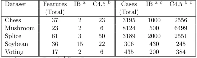
Table 2.7: Features and Training Sets Comparisons of Filter Based Feature Selection Algo-rithms and C4.5 Decision Tree
Dataset Features IB a C4.5b Cases IB a c C4.5b c
(Total) (Total)
Chess 37 2 23 3195 1000 2556
Mushroom 23 2 6 8124 500 6499
Splice 61 3 50 3189 2000 2551
Soybean 36 15 22 306 430 245
Voting 17 2 6 435 200 384
aInformation Based,bC4.5 Decision Tree, cIn training set
2.3.6 The Number of Features Reduced by C4.5 Decision Tree
Table 2.6 summarizes the number of features reduced by the decision tree classifier. The
percentages of feature reduction range between 25 and 73.91 and, on average, is about 55.6 percent for our four target datasets. Note that the Mushroom dataset has the highest percentage
of feature reduction as well as the highest learning time reduction and the highest accuracy
increases.
2.4
Discussion and Related Work
In this section, we will discuss feature selection techniques that have been applied during the construction of a Bayesian classifier.
Previous research on a filter feature selection method by Singh and Provan is based on information based metrics [31]. Their Info-AS algorithm incrementally adds a feature into
a set of selected features (originally an empty set) if it increases the value of information
based metric of that set of selected features. They then use the K2 algorithm to generate a BBN classifier based on these features. Three information based metrics were chosen for their
Table 2.8: Accuracy Comparison of Filter Based Feature Selection Algorithms and C4.5 De-cision Tree
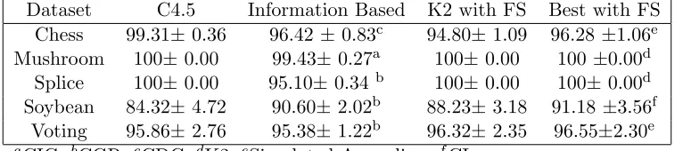
Dataset C4.5 Information Based K2 with FS Best with FS Chess 99.31±0.36 96.42 ±0.83c 94.80±1.09 96.28 ±1.06e Mushroom 100±0.00 99.43±0.27a 100±0.00 100±0.00d
Splice 100±0.00 95.10±0.34 b 100±0.00 100±0.00d Soybean 84.32±4.72 90.60±2.02b 88.23±3.18 91.18 ±3.56f
Voting 95.86±2.76 95.38±1.22b 96.32±2.35 96.55±2.30e aCIG,bCGR,cCDC,dK2, eSimulated Annealing,fCI
and the complement of Conditional Distance (CDC). Table 2.7 displays the total number of
features, the number of features selected by their information based method, and the number of features selected by our C4.5 decision tree method for all the datasets in their experiments.
Table 2.7 also shows the number of data points in the training sets for their information based
feature selection and our decision tree feature selection experiments. Note that while their experiments use arbitrary sizes of training sets, we use the 5-fold cross validation method.
The comparison of prediction accuracies between the two methods is shown in Table 2.8. Our
method has higher prediction accuracies for four out of the five datasets when comparing their best information based methods (metrics) on K2 algorithm with our best BBN learning
algorithms.
However, in order to account for our higher standard deviations and higher number of data points in the training sets, we perform extra experiments on Chess, Mushroom, Splice, and
Voting in a setting similar to their experiments in terms of the sizes of the training sets and
the number of experiments (30 trials). Note that we were not able to repeat the experiment on the Soybean dataset since the number of data points in the UCI repository has decreased from
630 to 306. For the Chess dataset, we achieved prediction accuracy of 97.06±0.52 (compared to their accuracy of 96.42±0.83) using a Simulated Annealing Algorithm. For the Mushroom dataset, we achieved prediction accuracy of 99.52± 0.36 (compared to their accuracy of 96.42
±0.83) using K2 algorithm. For the Splice dataset, we achieved prediction accuracy of 95.66±
0.58 (compared to their accuracy of 95.10±0.34) using K2 algorithm. For the Voting dataset, we achieved prediction accuracy of 96.15 ± 1.30 (compared to their accuracy of 95.38 ±1.22) using K2 algorithm.
One of the reasons for our method’s higher accuracies compared to information based
meth-ods is that the information based methmeth-ods suffer from the “curse of dimensionality.” These methods rely on being able to generate reliable probability estimates for the probability of
grows exponentially with the number of variables added even though the number of instances
that they see is limited by the size of the input. This means that many instantiations will have low values that could be very misleading. This could, in turn, lead to variables being selected
unnecessarily due to a misleading information value.
We avoid this problem by using the C4.5 decision tree algorithm to choose discriminatory
features because it uses a pruning technique once the full decision tree has been created. This
pruning is how C4.5 avoids overfitting the training data that has been seen. C4.5 uses the re-substitution error to determine the probability of seeing an error at a given level of the tree. If
there areN training cases that are covered by a leaf (in other words, the leaf is used to classify
N of the training cases) and there are E errors, then the resubstitution error is EN. This can also be viewed as seeing E events in N trials, which is modeled by the binomial distribution.
The probability of viewing an error, even if it is modeled by the binomial distribution, cannot
be determined exactly; however, it can be summarized by a pair of confidence limits. Given a confidence level, one can find an upper bound on the probability of finding an error. C4.5
equates the predicted error rate at a leaf with this upper bound on the probability. As a result,
it can replace an entire subtrees with a leaf as long as the predicted error rate of the new leaf is less than the sum size-weighted of the predicted error rates of the subtree that it will be
replacing. By using a confidence level, the C4.5 decision tree feature selection allows users the flexibility to choose this parameter to suit the degree of discriminability for their feature
selec-tion. C4.5 avoids the “curse of dimensionality” because it is pruned by using the resubstitution
error of a variable and comparing predicted error rates. In this way, it can more accurately decide the predictive power of an attribute.
In addition, our C4.5 decision tree feature selection method has the time complexity of
O(M NlogN) +O(N(logN)2) which is computationally less expensive thanO(M RN2(R+N))
of the information based method by Provan and Singh, whereM is the number of data points
and R is the maximum number of values for all features.
Kubat, Flotzinger, and Pfurtscheller used a decision tree to select a set of relevant features
and built a na¨ıve Bayesian classifier using only these selected features. Their experiment showed a promising result on Electroencephalography (EEG) signal classification by increasing the
ac-curacy by up to 30.35 percent (with an average of 19.33 percent) [32]. However, it is important
to note that on one of the datasets used for their experiments, a na¨ıve Bayesian classifier has a low accuracy (59.3 percent) which is improved (73.6 percent) when classified with a decision
tree. For datasets used in our experiments, the baseline prediction accuracy is already quite
was quite little room left for further improvements. We expect our method to perform (at least)
as well as their method, since a Bayesian classifier makes no assumption about the dependence relationship between features. In addition, our method has the advantage of learning the true
dependency relationships among features instead of assuming that they are independent of each
other, which is rarely true for real world applications.
Langley and Sage proposed the selective na¨ıve Bayesian classifier [33] using the idea of the
wrapper feature selection approach to implement a greedy sequential forward selection algorithm to wrap around a na¨ıve Bayesian classifier. Their experiment showed that the selective na¨ıve
Bayesian classifier is able to outperform a decision tree classifier on datasets that the na¨ıve
Bayesian classifier cannot. Singh and Provan extended this idea to a (non-na¨ıve) Bayesian classifier. The experiment showed that their method performed better than the selective and
non-selective (using full feature set) na¨ıve Bayesian classifiers. In fact, its performance was
com-parable to a Bayesian classifier constructed from the full feature set, and the network structure from their approach was easier to evaluate [34]. Since this experiment implements a feature
selection wrapper around K2 algorithm using Mushroom and Voting datasets, we are able to
compare their results with ours. For the Mushroom dataset, their accuracy ranges between 98.78 and 99.76 percent, which is less than our accuracy of 100 percent. For the Voting dataset,
their accuracy ranges between 94.2 and 96.44 percent, which is comparable to our accuracy of 96.32 percent. However, there is no report about the learning time of their method, though we
expect it to be higher than our method’s learning time since wrapper feature selection methods
are usually more expensive, computationally, than the filter method.
2.5
Conclusion
In this chapter we have proposed and implemented a feature selection method for BBNs which uses the discriminative power of the C4.5 decision tree algorithm to choose features to train on.
We tested both the running time and the prediction accuracy of our new method on four datasets
from the UCI Machine Learning Repository. We also compared the prediction accuracy of our feature selection method against an information based method on three additional datasets.
We found that our feature selection algorithm produced consistent reductions in the learning
time for a BBN as well as increasing the prediction accuracy of the resulting BBN in some cases. This characteristic of our feature selection algorithm is independently of the choice of
BBN learning algorithms. This means that we did not sacrifice prediction accuracy in order to decrease runtime. On the contrary, we showed that our method is able to effectively identify
we obtained is also quite significant. In most cases we were able to learn a BBN an order
Chapter 3
Iterative Decision Tree Feature
Knock-Out for Ensembles of
Bayesian Belief Network Classifiers
3.1
Problem and Proposed Solution
In Chapter 2, we proposed a filter-based feature selection technique to improve the performance
of Bayesian Belief Network (BBN) classifiers by reducing the learning time of BBNs without
sacrificing the prediction accuracy of the classifiers. We achieved this goal by using decision tree classifiers to identify a set of discriminating features and used only these features to construct
BBN classifiers. This method has many advantages: it is simple, fast, and scalable. In addition,
it can handle many types of features (continuous and multinomial). However, this method also has its limitations. One of its limitations is that this method may not be suitable for some real
world problem domains.
In some real world problem domains, learning a classifier model with high prediction accu-racy can be a difficult task due to the nature of data available. For example, in biology, recent
advances in DNA microarray technology allow the expression levels of thousands of genes
(fea-tures) to be measured simultaneously under different experimental conditions (samples) [35] [36], so the resulting data contains many more features than data points. These types of
prob-lems, where there are many more features than data points, are called underdetermined or unconstrained problems.
Underdetermined problems are hard to learn. One reason is that classifiers may take an
unreasonably large amount of computing power to analyze the large number of features in the
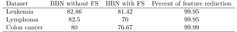
Table 3.1: Compare Prediction Accuracy for Underdetermined Problems
Dataset BBN without FS BBN with FS Percent of feature reduction
Leukemia 82.86 81.42 99.95
Lymphoma 82.5 70 99.95
Colon cancer 80 76.67 99.99
As a result, a learner may fail to construct high accuracy classifiers, because there is not enough data to distinguish between competitive but possibly inconsistent hypotheses [37].
To illustrate the difficulty of learning underdetermined problems, we performed an
experi-ment of building BBN classifiers with and without decision tree feature selection method from Chapter 2 on three microarray datasets. The result of this experiment is shown in Table 3.1.
We observe that although BBN classifiers with feature selection were able to reduce the number
of features in large percentages (which results in reducing the learning time), BBN classifiers with feature selection cannot achieve the same accuray as BBN classifiers without any feature
selection. Note that Table 3.3 displays the information about the datasets.
In this chapter, we are particularly interested in improving the performance of a BBN clas-sifier when the problems are underdetermined or underconstained. To address the issue of
learning underdetermined problems, we propose the Iterative Decision Tree Feature Knock-Out
for Ensembles of Bayesian Belief Network Classifiers (BBN-ITDT), an algorithm that incor-porates the concept of feature selection and ensemble methods to strengthen the classification
task.
Feature selection methods reduce the number of features, which result in decreasing in learning time. Learning time is one of the most challenging issues when learning with BBNs,
since the learning time of a BBN grows as fast as the size of search space. The size of the search space grows in the order ofO(2N2) [6], where N is the number of features.
Ensemble methods provide an advantage to the learning model by creating multiple
hy-potheses (each hypothesis corresponds to a base classifier) that combined together can improve the overall performance of a classifier. For BBN-ITDT algorithm, an ensemble method improves
the performance of a BBN classifier in two ways. First, it addresses the learning time issue of
BBNs because constructing many BBN classifiers, each one containing relatively few features, takes much less time than constructing one BBN classifier containing all features. Second,
ag-gregating predictions from an ensemble of classifiers has been shown to increase accuracy of an
ensemble classifier over a single classifier [38] [39] [40].
BBN-ITDT algorithm constructs an ensemble of BBN classifiers by using features selected
from a decision tree feature selection technique as described in Chapter 2. One problem here
for building an ensemble of classifiers. One solution to this problem is to perform a decision
tree feature selection technique in an iterative manner to produce a set of mutually exclusive feature sets. As a result, we are able to develop a technique for constructing an ensemble of
BBN classifiers that is suitable for underdetermined problems.
Before we describe BBN-ITDT algorithm in detail in Section 3.3, we would like to give some background information about ensemble methods in Section 3.2. Note that the background
information for feature selection methods can be found in Section 2.1.
3.2
Ensemble Methods
An ensemble of classifiers has been used to increase the prediction accuracy of single classifiers
by combining the predictions of several independent classifiers (base classifiers). In terms of machine learning, base classifiers form a hypothesis about the model of a target function. An
ensemble method makes its prediction by aggregating the prediction of many base classifiers
(often by incorporating some weighting schemes). An ensemble of classifiers improves the prediction accuracy of single classifiers by reducing the variance of the single classifier’s expected
error while the bias remain relatively unchanged.
Ensemble methods improve the prediction accuracy of a classifier by reducing the expected error of the classifier over all possible training sets of fixed size and a target function. Given
a fixed target function and a fixed size of training set, the expected error of a classifier is the
sum of the following three components: the target noise, the square of bias, and variance [38]. Target noise is an intrinsic property of classifiers. This value is the lower bound of the
expected error of any classifier, which is the expected error of a Bayes-optimal classifier.
The square of the “bias” is the measure of how closely a classifier’s average prediction (over all possible training sets) fits the target function. Typically, it is not feasible or practical to
enumerate all possible training sets, which makes it impossible to compute this value directly.
Variance is the measure of how divergent classifier’s predictions are among all the classifiers trained from all possible training sets. Here, we run into the problem of having to enumerate
all possible training sets in order to calculate this value exactly.
Most research on ensemble methods has been dedicated to improving the prediction accuracy of classifiers. In the next paragraphs, we will focus on four areas of research in greater detail.
First, many studies are interested in applying an ensemble method to “weak” and/or “unstable”
single classifiers. Second, some research studies are more interested in understanding how ensemble methods can reduce the expected error of classifiers. Third, some studies try to
take advantage of ensemble methods when the available data is problematic, such as having underdetermined or high-dimensional data. Last, some researchers are interested in improving
describe methods from each of these categories.
3.2.1 Ensemble Methods for “Weak” or “Unstable” Classifiers
Ensemble methods have been successfully applied to many single classifiers in order to improve their prediction accuracy. A classifier is said to be “unstable” if a small change in that classifier’s
training data will produce a large change in that classifier’s predictions [41]. One characteristic
of “unstable” classifiers is high variance [42]. Examples of “unstable” classifiers are decision tree classifiers and neural networks. Examples of “stable” classifiers are linear discriminant
analysis (LDA) and nearest neighbor[42].
A “weak” classifier is a classifier that makes prediction only slightly better than random
guessing. An example of a “weak” classifier is a decision stump. Note that a “weak” classifier is
not the same as an “unstable” classifier. For example, decision tree is a “strong” but “unstable” classifier or nearest neighbor is a “weak” but “stable” classifier.
There are three well-known ensemble methods, bagging, boosting, and random forests, and
each method has been applied to many types of classifiers; however, not all classifiers that have been coupled with ensemble methods are proven to be “weak” or “unstable.” Nonetheless,
ensemble methods have been shown to improve the prediction accuracy in most of them.
Bagging, also known as bootstrap aggregating [41], is an ensemble technique, in which an ensemble of classifiers is created by randomly sampling (with replacement) the original training
set to create multiple training sets. These training sets are then used to train the ensemble of
classifiers. The ensemble classifier makes its prediction by having each classifier in the ensemble make a prediction and then taking the majority value of these base predictions. Bagging can
improve the prediction accuracy by reducing the variance of an “unstable” classifier [38]. Many
research studies show that bagging can improve the prediction accuracy of multilayer perceptron [43], radial basis function networks [43], na¨ıve BBN [43] [44], BBN [43], SVM [39], decision trees
[43] [44] [45] [38],nearest neighbor [38], and neural networks [46] [45] .
Boosting is an ensemble technique that is based on the idea of “weak learnability” [47]. Boosting builds an ensemble of classifiers by giving various distributions of the training set to
a (“weak”) learning algorithm. This method differs from bagging in the sense that boosting is
an iterative process. In the first iteration, the boosting method is given an initial distribution for selecting data points from the original training set in order to construct one classifier.
Typically this distribution is uniform, meaning that there is an equal probability of sampling
each data point in the original training set. This classifier is used to evaluate the data points in the training set. The data points that are misclassified are given higher probability of being
Boosting can reduce the expected error of classifiers by reducing the bias, although boosting
will typically increase the variance. For example, a study shows that boosting can increase variance in “stable” classifiers, such as a na¨ıve BBN classifier [38]. Boosting has been applied to
many classifiers. Examples include multilayer perceptron [43], radial basis function network [43],
na¨ıve BBN [43], BBN [43], SVM [39], and decision tree [43]. In addition boosting (AdaBoost) has been used for feature selection [48].
Random forests [49] are constructed from the entire set of data points; however, only a
subset of the features from the original training set is used. For each classifier, the features in the training set are randomly selected without replacement. The final prediction is usually
the result of voting similar to bagging. Random forests improve the prediction accuracy of a
classifier by reducing the variance. Random forests have been applied to base classifiers such as a multilayer perceptrons [43], radial basis function networks [43], na¨ıve BBNs [43] [41], BBNs
[43], SVMs [50] [39] [41], and decision trees [51] [43]. In addition, random forests have been
used for feature selection as well [51].
3.2.2 Ensemble Method for Reducing the Expected Error
Since target noise is constant, many research studies on ensemble methods have been focusing
on reducing the bias and/or the variance of a classifier. However, it is often the case that there is a trade-off between reducing the bias and reducing the variance. For example, increasing
the size of an ensemble (i.e., the number of base classifiers) often results in decreasing the bias
while increasing the variance.
A bias is introduced to a learning algorithm when it chooses one hypothesis over another
rather than staying strictly consistent with the training data points [38]. Two varieties of
bias (related to machine learning) are “absolute bias” and “relative bias.” “Absolute bias” is related to how the learning algorithm chooses the family of functions to represent its hypotheses.
“Absolute bias” can either be appropriate (contains a good approximator) or inappropriate
(does not contain a good approximator) of the target function [38]. “Relative bias” is related to how the learning algorithm narrows down the hypotheses within the chosen function. “Relative
bias” can either be too strong because it prefers poorer hypotheses, or too weak because it
considers too many hypotheses [38].
In relation to bias and variance, if the “absolute bias” is inappropriate and/or the “relative
bias” is too strong, then the algorithm will have high bias. If the “relative bias” is too weak,
then the algorithm will have high variance. So a good learning algorithm is the one with appropriate “absolute bias” and the right strength of “relative bias” [38].